The Hairy Chart, in R

Project

Data Visualization

The federal funds rate and its forecast (hairy) paths, replicated in R.

Author

Curtis Kephart

Published

Oct 17, 2026

This notebook walks through how to access the data and replicate the federal funds “hairy chart” in R. The hairy chart plots the federal funds rate over time and, at each past date, the path the rate was then expected to take, drawn as a thin line, or “hair”.

We’ll load the federal funds target rate, then four sources of expected paths: the Treasury forward curve, options on SOFR futures, the FOMC’s median projection, and the Survey of Professional Forecasters. Each source is described, sourced, loaded and plotted on its own, followed by a simpler forecast a reader suggested, the 2-year Treasury yield. Then the four sources go on one plot, and a forecast evaluation scores them.

Each section summarizes how its data was downloaded and cleaned; the full pipeline, with a README on rebuilding the data, is in the repo’s scripts/ folder, and the cleaned files the notebook reads are in data/.

Setup

Packages, the color palette, plot theme, the per-source labels and captions, and helper functions that the tables and plots below reuse.

Code

library(dplyr)
library(readr)
library(ggplot2)
library(scales)
library(gt)

RATE <- "#0B1B4A"
INK <- "#1B3A6B"
INK_SOFT <- "#5C7599"
GRID <- "#C9D6E6"
BG <- "#FFFFFF"

# Checked for separation under normal and color-blind vision.
pal <- c(
  treasury_forward = "#2E7DBF",
  options_implied  = "#C8102E",
  sep_median       = "#E08A1E",
  spf_median       = "#8C1A8C"
)

src_label <- c(
  treasury_forward = "Treasury Forward Curve",
  options_implied  = "Options-Implied (SOFR)",
  sep_median       = "FOMC Median Projection",
  spf_median       = "Professional Forecasters"
)

# Named in the subtitle alongside the target rate.
src_phrase_subtitle <- c(
  treasury_forward = "Treasury forward curves",
  options_implied  = "options-implied expected SOFR paths",
  sep_median       = "FOMC median projected rate paths",
  spf_median       = "professional forecasters' expected rate paths"
)

# Caption sources. Every plot shows the target rate, published by the Federal
# Reserve Board and retrieved through FRED, alongside its own hair source.
target_src <- "Federal Reserve Board via the St. Louis Fed's FRED (target rate)"

src_caption <- c(
  treasury_forward = "Federal Reserve Board, GSW nominal yield curve",
  options_implied  = "Federal Reserve Bank of Atlanta, Market Probability Tracker",
  sep_median       = "Federal Reserve Board, Summary of Economic Projections",
  spf_median       = "Federal Reserve Bank of Philadelphia, Survey of Professional Forecasters"
)

theme_hairy <- function() {
  theme_minimal(base_size = 12) +
    theme(
      plot.background = element_rect(fill = BG, color = NA),
      panel.background = element_rect(fill = BG, color = NA),
      panel.grid.minor = element_blank(),
      panel.grid.major.x = element_blank(),
      panel.grid.major.y = element_line(color = GRID, linewidth = 0.4),
      axis.text = element_text(color = INK_SOFT),
      axis.ticks.x = element_line(color = INK_SOFT, linewidth = 0.3),
      axis.ticks.length.x = unit(4, "pt"),
      axis.minor.ticks.length.x = rel(0.5),
      axis.title = element_blank(),
      plot.title = element_text(color = INK, face = "bold", size = 15),
      plot.subtitle = element_text(color = INK_SOFT, size = 10.5),
      plot.caption = element_text(color = INK_SOFT, size = 8, hjust = 0),
      legend.title = element_blank(),
      legend.text = element_text(color = INK, size = 9.5)
    )
}

# Font family and size inherit from the page, so the tables match the body
# text wherever the notebook is embedded.
gt_basic <- function(d) {
  gt(d) |>
    tab_options(
      table.font.names = "inherit",
      table.font.size = "inherit",
      table.background.color = BG,
      column_labels.font.weight = "bold",
      data_row.padding = px(5),
      table.border.top.style = "none"
    )
}

# One row per source: how many hairs, how many points each, how far apart the
# points are, and how much time a typical hair covers.
hair_summary <- function(d) {
  per_hair <- d |>
    arrange(as_of, target_date) |>
    group_by(as_of) |>
    summarise(
      points = n(),
      span = as.numeric(max(target_date) - min(target_date)),
      step = median(as.numeric(diff(target_date))),
      .groups = "drop"
    )
  step <- median(per_hair$step, na.rm = TRUE)
  tibble(
    Hairs = nrow(per_hair),
    Points = nrow(d),
    `Points per hair` = median(per_hair$points),
    `Point spacing` = if (step < 45) "Monthly" else if (step < 120) "Quarterly" else "Yearly",
    `Typical span (months)` = round(median(per_hair$span) / 30.44)
  )
}

# Forecaster values are calendar-quarter averages, so those hairs are drawn as
# steps, each value held across its quarter. The other sources are joined by
# straight lines.
step_sources <- "spf_median"

# Plot-ready hairs for one source. Each hair starts on the target line at its
# forecast date, reading the target one day later because FRED dates a change
# from the day it takes effect, so a forecast made at an FOMC meeting starts
# from that meeting's decision. Step sources get one row per quarter start,
# clipped to the forecast date, plus the last quarter's end. Plotting only;
# hairs.csv and the tables hold source points alone.
hair_path <- function(h, src) {
  anchors <- h |>
    distinct(as_of) |>
    mutate(
      target_date = as_of,
      rate_pct = ffr$target_mid[match(as_of + 1, ffr$date)]
    ) |>
    filter(!is.na(rate_pct))
  points <- h |> select(as_of, target_date, rate_pct)
  if (src %in% step_sources) {
    last <- points |> group_by(as_of) |> slice_max(target_date, n = 1) |> ungroup()
    points <- bind_rows(
      points |> mutate(target_date = pmax(lubridate::floor_date(target_date, "quarter"), as_of)),
      last |> mutate(target_date = lubridate::ceiling_date(target_date, "quarter"))
    )
  }
  bind_rows(anchors, points)
}

hair_geom <- function(src, ...) {
  if (src %in% step_sources) geom_step(direction = "hv", ...) else geom_line(...)
}

# Year axis: a label on round years every `every` years, a small tick each year.
scale_x_years <- function(from, to, every = 5) {
  years <- function(k) {
    y0 <- ceiling(as.integer(format(from, "%Y")) / k) * k
    as.Date(sprintf("%d-01-01", seq(y0, as.integer(format(to, "%Y")), by = k)))
  }
  scale_x_date(
    breaks = years(every), minor_breaks = years(1),
    labels = label_date("%Y"), guide = guide_axis(minor.ticks = TRUE)
  )
}

# The target rate, reused by every plot below: the target, or the midpoint of
# the target range, as a heavy line.
rate_line <- function(d) {
  geom_line(
    data = d, aes(date, target_mid),
    color = RATE, linewidth = 1.0, lineend = "round"
  )
}

plot_source <- function(src, pad_years = 1) {
  h <- hairs |> filter(source == src)
  x0 <- min(h$as_of) - 365 * pad_years
  x1 <- max(h$target_date) + 180
  d <- ffr |> filter(date >= x0, date <= x1)
  y_max <- max(c(h$rate_pct, d$target_mid), na.rm = TRUE) * 1.08

  # Hair counts differ by a factor of twenty between sources, so a fixed alpha
  # leaves the SEP plot faint and the options plot a solid block.
  n <- n_distinct(h$as_of)
  a <- max(0.08, min(0.55, 60 / n))

  # Labels every 5, 2 or 1 years depending on how much time the plot spans.
  span <- as.numeric(x1 - x0) / 365.25
  every <- if (span > 20) 5 else if (span > 8) 2 else 1

  ggplot() +
    hair_geom(
      src, data = hair_path(h, src), mapping = aes(target_date, rate_pct, group = as_of),
      color = pal[[src]], alpha = a, linewidth = 0.4, lineend = "round"
    ) +
    rate_line(d) +
    scale_x_years(x0, x1, every) +
    scale_y_continuous(labels = label_number(suffix = "%")) +
    coord_cartesian(xlim = c(x0, x1), ylim = c(-0.3, y_max)) +
    labs(
      title = src_label[[src]],
      subtitle = paste("Federal funds target rate and", src_phrase_subtitle[[src]]),
      caption = paste0("Sources: ", src_caption[[src]], "; ", target_src, ".")
    ) +
    theme_hairy()
}

Data

Federal Funds Target Rate

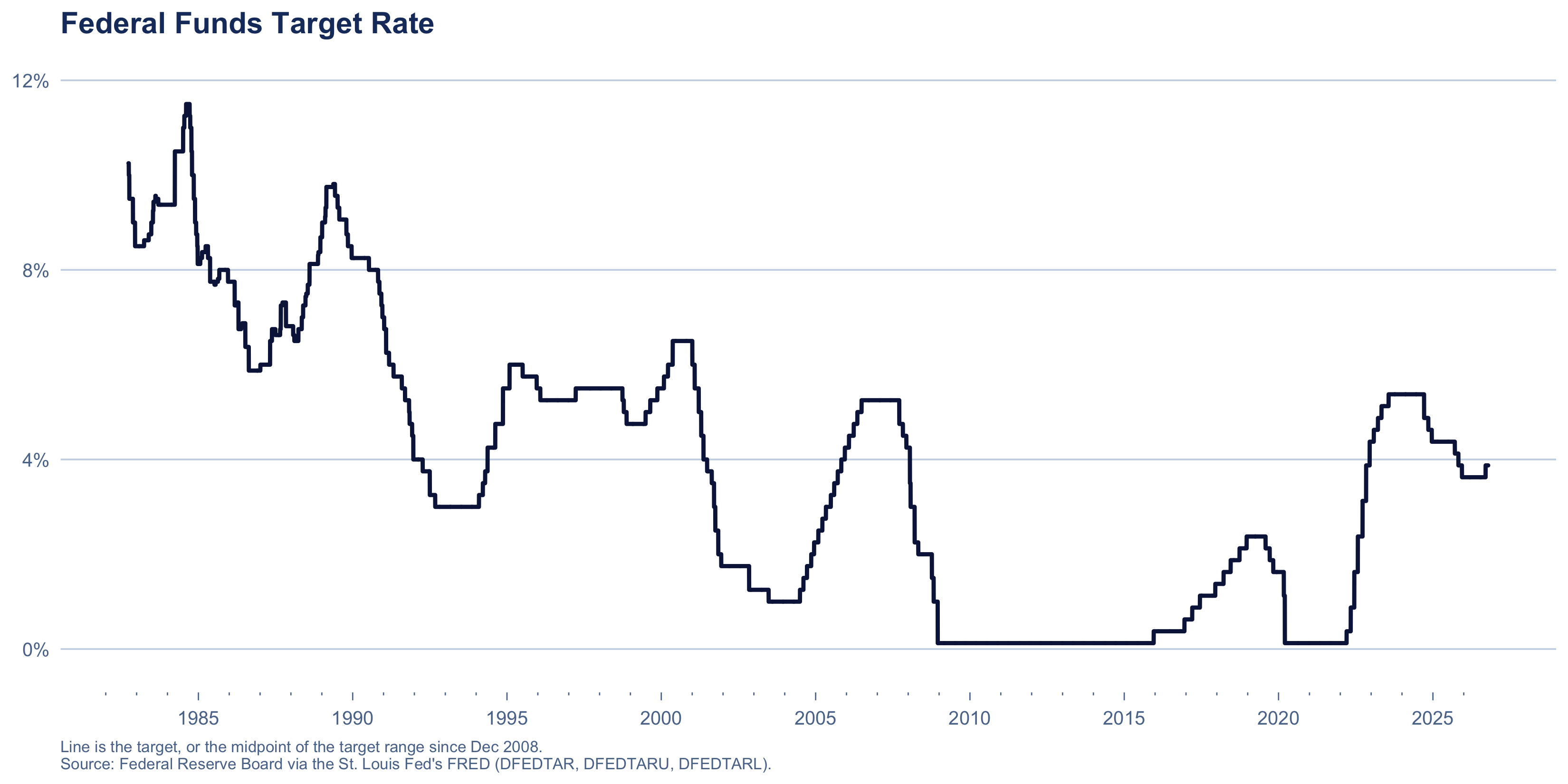
In a sense, this is the head from which all the hairs grow.

Downloaded from the FRED database, series DFEDTAR, DFEDTARL and DFEDTARU, by fetch_fred.py. The series are assembled by build_dataset.py, which splices the pre-2008 single target into the range columns so target_lo, target_hi and target_mid run continuously across the December 2008 regime change.

Source Detail: The FOMC Target (click to expand)

The rate the Federal Open Market Committee announces it is aiming for. A single number until December 2008, a quarter-point range from then on. The New York Fed: “The Federal Open Market Committee establishes the target rate, or range, for trading in the federal funds market.”

FRED DFEDTAR is the single target, 27 September 1982 to 15 December 2008. DFEDTARL and DFEDTARU are the lower and upper limits of the range from 16 December 2008, when the Committee cut to 0 to 0.25 percent and has used a range ever since. Verified at the join: DFEDTAR ends 2008-12-15 at 1.00, DFEDTARL/DFEDTARU begin 2008-12-16 at 0.00/0.25.

Values before 1994 are a reconstruction: the FOMC began announcing its target decisions in February 1994, and FRED’s series notes say the 1982 to 1993 values come from Thornton (2005), a Federal Reserve Bank of St. Louis working paper.

Citations.

https://fred.stlouisfed.org/series/DFEDTAR
https://fred.stlouisfed.org/series/DFEDTARU
https://fred.stlouisfed.org/series/DFEDTARL
Thornton, Daniel L. (2005), “A New Federal Funds Rate Target Series: September 27, 1982 - December 31, 1993”, Federal Reserve Bank of St. Louis
https://www.newyorkfed.org/markets/reference-rates/effr

Code

ffr <- read_csv("../data/fed_funds_rate.csv", show_col_types = FALSE)

ffr |>
  summarise(
    From = format(min(date), "%b %Y"),
    To = format(max(date), "%b %Y"),
    Days = n(),
    `Target changes` = sum(target_mid != lag(target_mid), na.rm = TRUE),
    `Range era begins` = format(min(date[target_lo != target_hi]), "%d %b %Y")
  ) |>
  gt_basic()

From	To	Days	Target changes	Range era begins
Sep 1982	Oct 2026	16092	185	16 Dec 2008

Code

ggplot() +
  rate_line(ffr) +
  scale_x_years(min(ffr$date), max(ffr$date)) +
  scale_y_continuous(labels = label_number(suffix = "%")) +
  coord_cartesian(ylim = c(-0.3, 12)) +
  labs(
    title = "Federal Funds Target Rate",
    caption = paste(
      "Line is the target, or the midpoint of the target range since Dec 2008.",
      "\nSource: Federal Reserve Board via the St. Louis Fed's FRED (DFEDTAR, DFEDTARU, DFEDTARL)."
    )
  ) +
  theme_hairy()

Hairs

“Hairs” here are the predicted paths of the federal funds rate, from different sources. All four live in one tidy table, loaded once here and described one at a time below.

Code

hairs <- read_csv("../data/hairs.csv", show_col_types = FALSE) |>
  mutate(
    source = factor(source, levels = names(pal)),
    across(c(as_of, target_date), as.Date)
  )


hairs |>
  group_by(source) |>
  summarise(
    Hairs = n_distinct(as_of),
    Points = n(),
    From = format(min(as_of), "%b %Y"),
    To = format(max(as_of), "%b %Y"),
    .groups = "drop"
  ) |>
  mutate(Source = src_label[as.character(source)], .keep = "unused", .before = 1) |>
  gt_basic()

Source	Hairs	Points	From	To
Treasury Forward Curve	264	9504	Feb 1994	Sep 2026
Options-Implied (SOFR)	893	10217	Mar 2023	Oct 2026
FOMC Median Projection	44	155	Sep 2015	Sep 2026
Professional Forecasters	176	880	Nov 1982	Aug 2026

Treasury Forward Curve

Source Detail: GSW Nominal Yield Curve (click to expand)

What the Treasury bond market implies about future short rates, backed out daily by Federal Reserve Board staff from a smooth curve fitted across the whole maturity spectrum.

The Board describes the dataset as “smoothed yields on hypothetical Treasury securities that can be easily compared across maturities and over time, from 1961 to the present”. Its model “stipulates that the shape of the yield curve on any given date can be adequately captured by a set of six parameters”, estimated “by minimizing the discrepancy between the fitted Svensson yield curve and observed market yields”. Before 1980, “the Nelson-Siegel model—a model with fewer parameters—was used”.

On what goes into the fit: “only the coupon securities (Treasury notes and bonds) are used”; “on-the-run and first-off-the-run Treasury notes and bonds are not used”; and “Treasury bills and Treasury floating rate notes (FRNs) are not used”.

It is not an official statistic. The Board calls it “a staff research product and not an official statistical release”. A forward rate is the expected future short rate plus a term premium, so the hairs aren’t a pure expectations path: they can sit a little above or below it. And because bills are excluded and the curve is a six-parameter analytic function, the hairs are smooth by construction: they cannot show the discrete steps at FOMC meetings that market data pricing individual meetings shows.

Citations.

https://www.federalreserve.gov/data/nominal-yield-curve.htm
Gürkaynak, Sack and Wright (2006), FEDS 2006-28, https://www.federalreserve.gov/pubs/feds/2006/200628/200628pap.pdf
Published in Journal of Monetary Economics 54(8), 2007, 2291-2304

Downloaded from the Federal Reserve Board’s nominal yield curve data, as feds200628.csv. For each day, the file includes the six parameters of the fitted curve described in the source detail above. build_gsw_hairs.py plugs them into the formula for the instantaneous forward rate, the overnight rate the curve implies n years ahead:

\[ \begin{aligned} f(n) = {} & \beta_0 + \beta_1 e^{-n/\tau_1} \\ & + \beta_2 \tfrac{n}{\tau_1} e^{-n/\tau_1} + \beta_3 \tfrac{n}{\tau_2} e^{-n/\tau_2} \end{aligned} \]

The file also lists the forward rates themselves, but only for whole years ahead, so the script computes them for every month ahead; at whole years, the two agree. The results stay continuously compounded, which is close to how an overnight rate like fed funds is quoted.

build_dataset.py then samples the curve on FOMC meeting dates, taken from the Board’s meeting calendars by fetch_fomc_dates.py. build_long_hairs.py writes the same hairs out to 120 months, for the length comparison below; the Board publishes the curve out to 30 years.

Code

treasury_forward <- hairs |> filter(source == "treasury_forward")

# The same hairs uncapped, for the length comparison only.
treasury_long <- read_csv("../data/treasury_forward_120m.csv", show_col_types = FALSE)


hair_summary(treasury_forward) |>
  gt_basic()

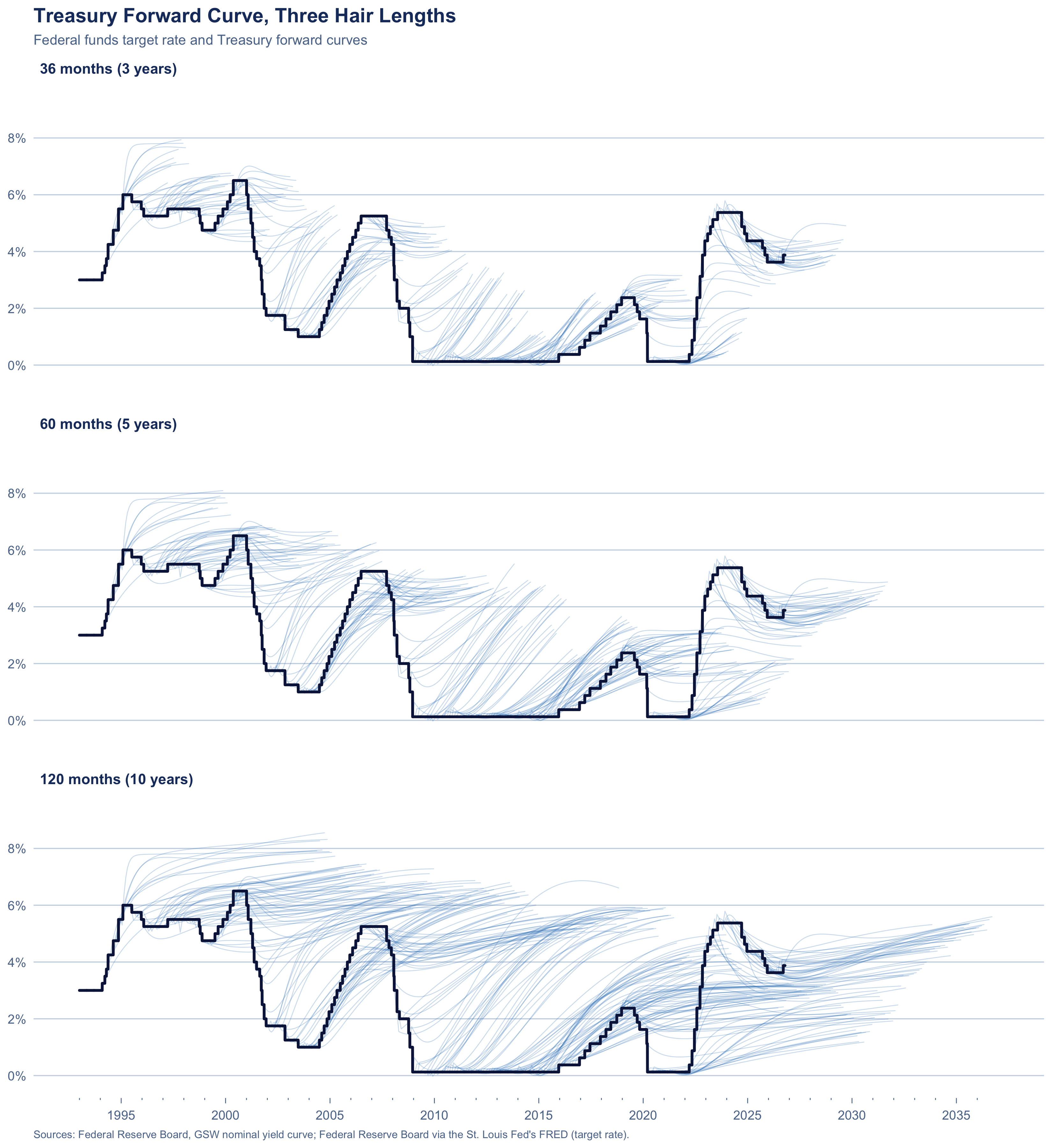
Hairs	Points	Points per hair	Point spacing	Typical span (months)
264	9504	36	Monthly	35

What longer hairs for this series would look like, cut at 36, 60 and 120 months:

Code

cuts <- c(36, 60, 120)

long_cut <- lapply(cuts, function(k) {
  hair_path(treasury_long |> filter(horizon_months <= k), "treasury_forward") |>
    mutate(length = sprintf("%d months (%g years)", k, k / 12))
}) |>
  bind_rows() |>
  mutate(length = factor(length, levels = unique(length)))

ggplot() +
  geom_line(
    data = long_cut, aes(target_date, rate_pct, group = as_of),
    color = pal[["treasury_forward"]], alpha = 0.25, linewidth = 0.3, lineend = "round"
  ) +
  rate_line(ffr |> filter(date >= as.Date("1993-01-01"))) +
  facet_wrap(~length, ncol = 1) +
  scale_x_years(as.Date("1993-01-01"), as.Date("2036-12-31")) +
  scale_y_continuous(labels = label_number(suffix = "%"), breaks = seq(0, 10, 2)) +
  coord_cartesian(
    xlim = as.Date(c("1993-01-01", "2036-12-31")),
    ylim = c(-0.3, 9.5)
  ) +
  labs(
    title = "Treasury Forward Curve, Three Hair Lengths",
    subtitle = "Federal funds target rate and Treasury forward curves",
    caption = paste0("Sources: ", src_caption[["treasury_forward"]], "; ", target_src, ".")
  ) +
  theme_hairy() +
  theme(
    strip.text = element_text(color = INK, face = "bold", hjust = 0, size = 11),
    panel.spacing.y = unit(1.2, "lines")
  )

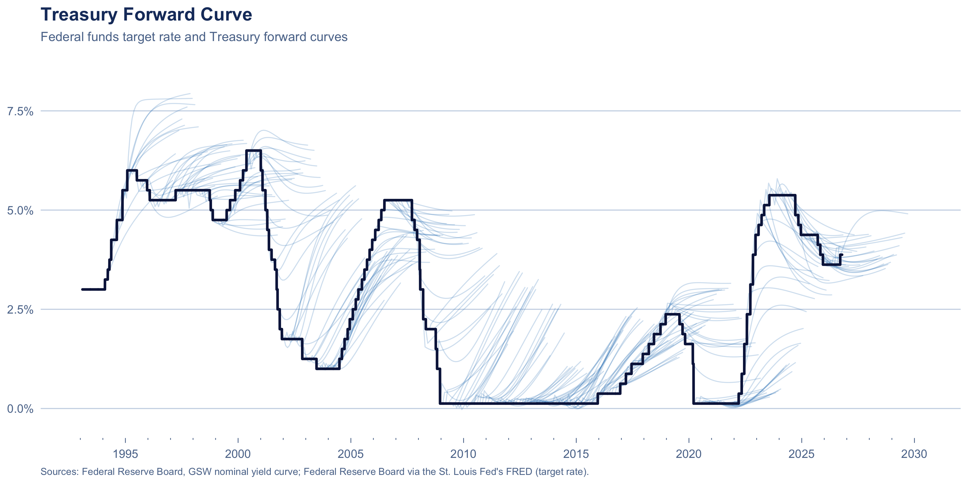
Hairs are cut at 36 months for legibility. I personally like the long fan rising out of the 2009 to 2015 floor: the market repeatedly pricing a liftoff that didn’t come until December 2015.

Code

plot_source("treasury_forward")

Options-Implied (SOFR)

Source Detail: Atlanta Fed Market Probability Tracker (click to expand)

What options traders are collectively betting, as a full probability distribution over where the overnight rate will average in a future three-month window.

From the data dictionary shipped inside the file: “The Market Probability Tracker uses Chicago Mercantile Exchange (CME) 3-month SOFR options to estimate the probability ditributions [sic] implied by their prices and specified reference window.” Their guide adds that it “transforms options on SOFR futures prices into probability distribution values”.

Two fields are used. reference_start is the “Start date of the 3-month window referenced by CME 3-month SOFR contracts”. Rate: mean is “The rate, in basis points, associated with the mean of the estimated distribution for a given reference window”.

The underlying rate is SOFR, published by the Federal Reserve Bank of New York: a broad measure of the cost of borrowing cash overnight collateralized by US Treasury securities. That makes it a secured rate, where the federal funds rate is unsecured lending between banks; the two are close but not identical. An option-implied distribution is risk-neutral, so it is what traders expect weighted by how much they care about being wrong each way, not literally what they expect. It starts in March 2023.

Each point comes from its own window’s option prices rather than from one fitted curve, but as a three-month average weighted across possible outcomes it does not resolve individual FOMC meetings.

Citations.

https://www.atlantafed.org/research-and-data/data/market-probability-tracker
https://www.atlantafed.org/research-and-data/data/market-probability-tracker/what-to-know
https://www.newyorkfed.org/markets/reference-rates/sofr
Estimation code published as mpt_source.zip on the tracker page

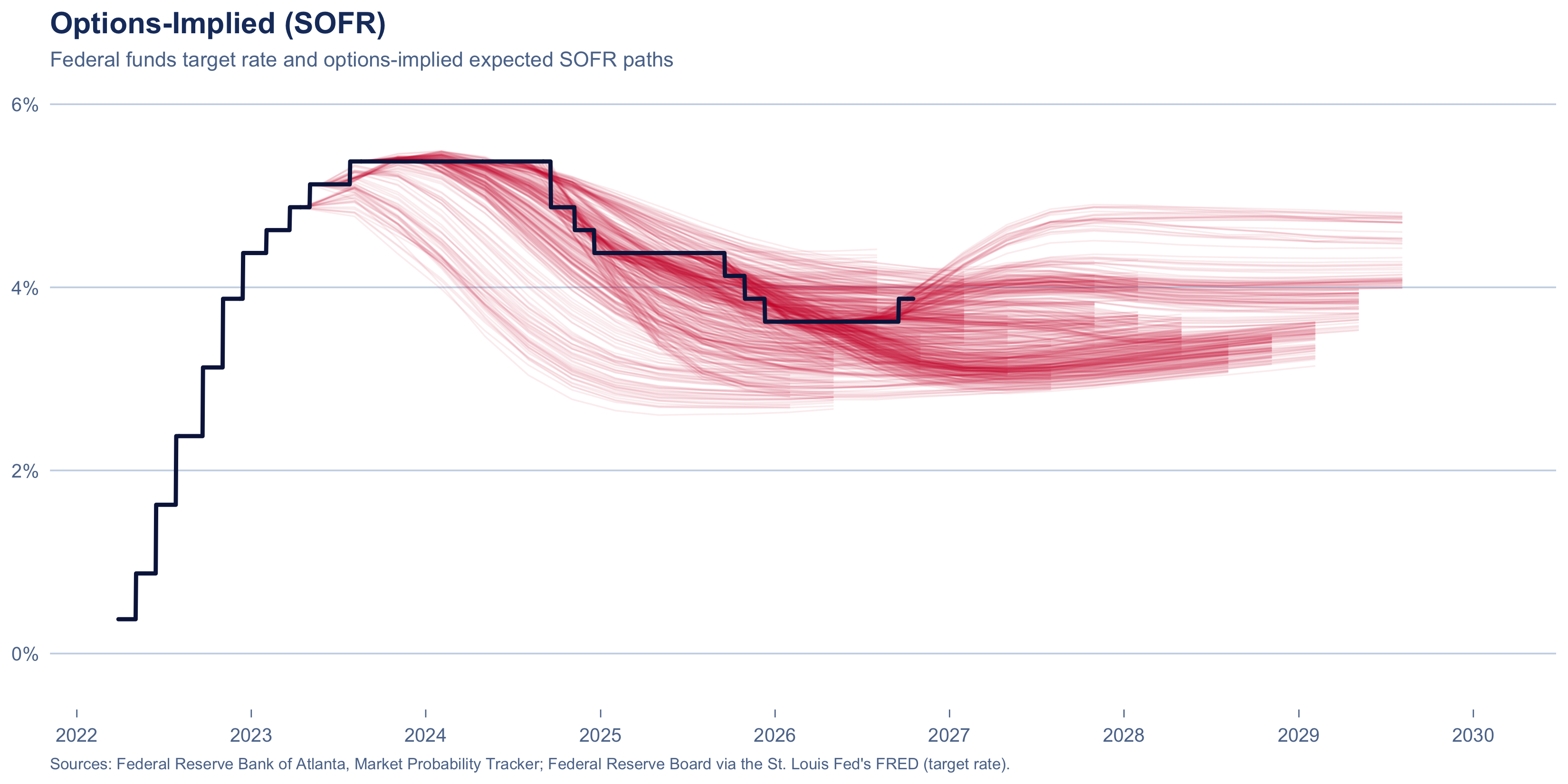
These hairs come from options on SOFR (Secured Overnight Financing Rate) futures. A SOFR futures contract settles on where SOFR averages over a future three-month window; options on that contract, across a range of strike prices, imply a probability distribution for the average. The Atlanta Fed estimates those distributions daily, and each hair is the mean of the distribution for each successive window, as of one day.

Downloaded from the Federal Reserve Bank of Atlanta’s Market Probability Tracker, as mpt_histdata.xlsx. build_dataset.py takes the DATA sheet, keeps field == "Rate: mean", divides by 100 to turn basis points into percent, and places each point at the midpoint of its reference window, which is reference_start plus 45 days.

Code

options_implied <- hairs |> filter(source == "options_implied")

hair_summary(options_implied) |>
  gt_basic()

Hairs	Points	Points per hair	Point spacing	Typical span (months)
893	10217	11	Quarterly	30

Code

plot_source("options_implied")

FOMC Median Projection

Source Detail: The Summary of Economic Projections (click to expand)

Four times a year each of the Federal Reserve’s senior policymakers writes down where they think the federal funds rate should be at the end of each of the next few years. This is the middle answer.

The table is titled “Economic projections of Federal Reserve Board members and Federal Reserve Bank presidents, under their individual assumptions of projected appropriate monetary policy”: all 7 Governors plus all 12 Reserve Bank presidents. That is wider than the Committee’s voting membership: the Board says the Committee “consists of twelve members”, namely “the seven members of the Board of Governors of the Federal Reserve System; the president of the Federal Reserve Bank of New York; and four of the remaining eleven Reserve Bank presidents, who serve one-year terms on a rotating basis”. Staff produce a separate forecast, the Tealbook, released only after five years.

From the table notes: “The projections for the federal funds rate are the value of the midpoint of the projected appropriate target range for the federal funds rate or the projected appropriate target level for the federal funds rate at the end of the specified calendar year or over the longer run.” And: “For each period, the median is the middle projection when the projections are arranged from lowest to highest.”

It is not a forecast. The row is labeled “Memo: Projected appropriate policy path”, and projections rest on each participant’s “assessment of appropriate monetary policy”. Normative, conditional on each person’s own outlook, and never voted on.

Only 44 of 59 releases give a median. The median column was introduced with the September 2015 SEP; before that the table shows a central tendency and range only, and the dots exist solely as a figure.

Citations.

https://www.federalreserve.gov/monetarypolicy/files/fomcprojtabl{YYYYMMDD}.pdf
https://www.federalreserve.gov/monetarypolicy/fomc.htm
https://fred.stlouisfed.org/series/FEDTARMD
https://www.federalreserve.gov/monetarypolicy/fomc_projectionsfaqs.htm

Downloaded from the Federal Reserve Board, one projection-table PDF per meeting, by fetch_forecasts.py. parse_sep.py reads the median row from each table; build_dataset.py dates each value to 31 December of its year and drops the longer-run value. Cross-checked against FRED.

Code

sep_median <- hairs |> filter(source == "sep_median")

hair_summary(sep_median) |>
  gt_basic()

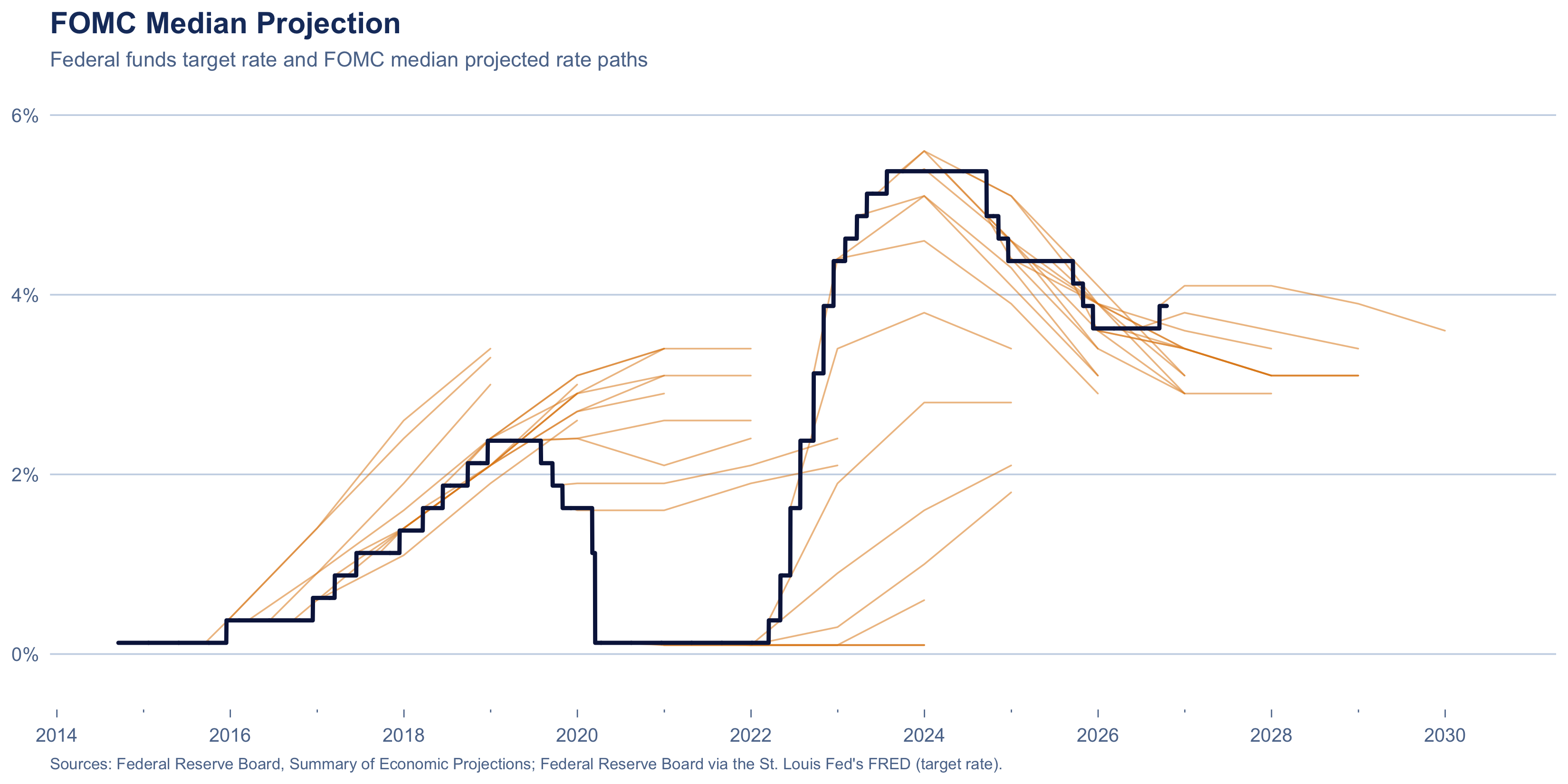
Hairs	Points	Points per hair	Point spacing	Typical span (months)
44	155	4	Yearly	36

Four points per hair at most, one per projection year, dated to 31 December.

Code

plot_source("sep_median")

Professional Forecasters

Source Detail: Survey of Professional Forecasters (click to expand)

Every quarter the Philadelphia Fed asks a few dozen professional forecasters where the three-month Treasury bill rate will be over the next five quarters, and publishes the median.

The Philadelphia Fed describes it as “the oldest quarterly survey of macroeconomic forecasts in the United States. The survey began in 1968 and was conducted by the American Statistical Association and the National Bureau of Economic Research. The Federal Reserve Bank of Philadelphia took over the survey in 1990.” Individual responses are “kept confidential by using identification numbers”.

The survey asks about the bill rate, not the federal funds rate, but the two track each other closely: a three-month bill pays roughly what investors expect overnight rates to average over its three months. The bill normally sits a little below fed funds, so a forecast of the bill rate works as a rough forecast of the policy rate that runs slightly low.

Citations.

https://www.philadelphiafed.org/surveys-and-data/real-time-data-research/survey-of-professional-forecasters
Documentation PDF: variable definitions p.10, horizon numbering p.20, survey timing p.7

Downloaded from the Federal Reserve Bank of Philadelphia’s Survey of Professional Forecasters page, as median_tbill_level.xlsx, by fetch_forecasts.py. build_dataset.py drops TBILL1, the quarter before the survey, whose value forecasters already know, so horizons run from the current quarter (TBILL2) to four quarters ahead (TBILL6). It dates each hair at the response deadline, the middle of the quarter’s second month, and drops the five surveys from before September 1982, when the target series begins.

Code

spf_median <- hairs |> filter(source == "spf_median")


hair_summary(spf_median) |>
  gt_basic()

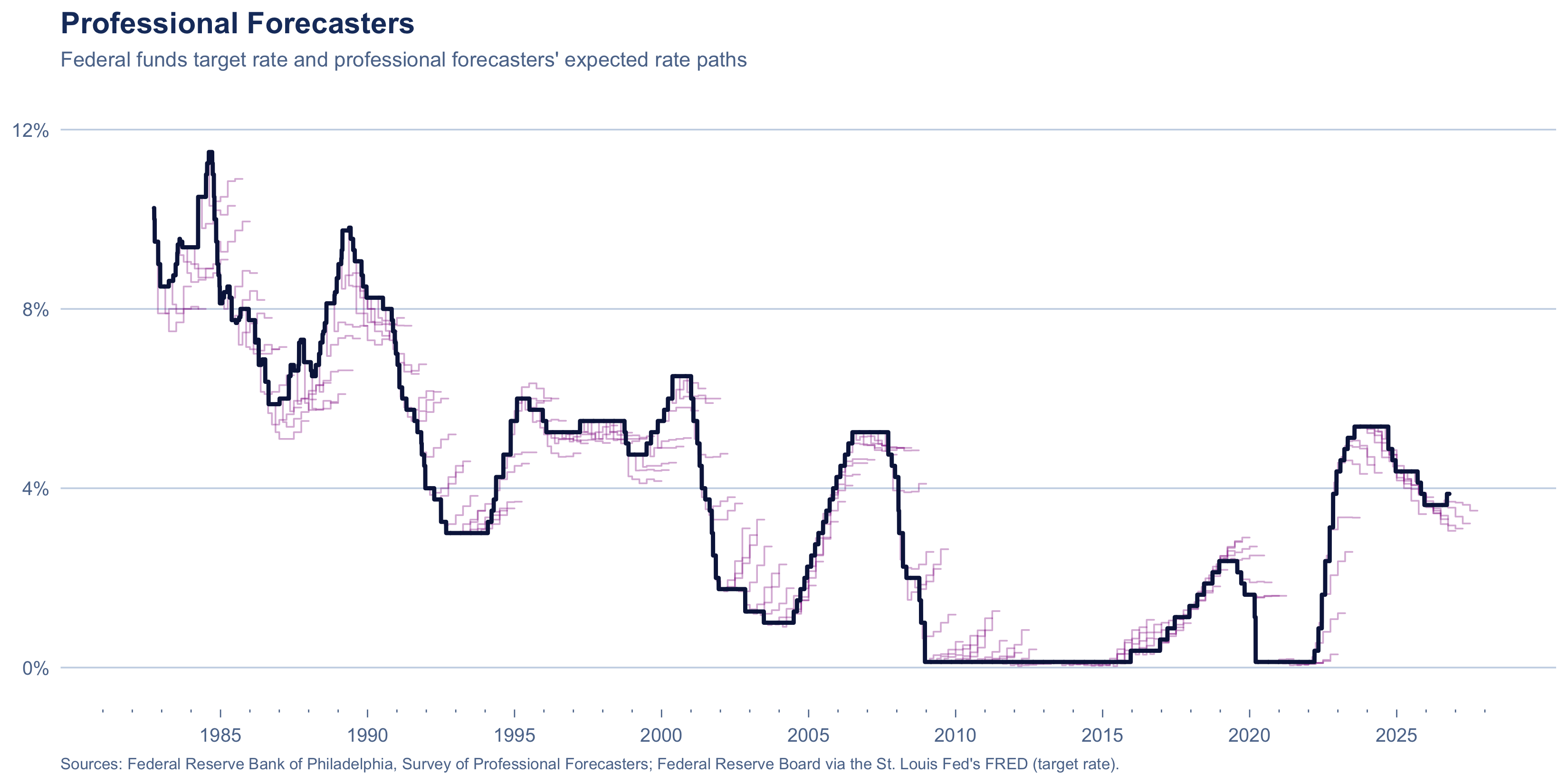
Hairs	Points	Points per hair	Point spacing	Typical span (months)
176	880	5	Quarterly	12

Five quarterly averages per hair, each drawn as a step across its quarter, covering about a year. The only one of the four reaching the 1980s.

Code

plot_source("spf_median")

2-Year Treasury Yield with Offset

I received a comment suggesting a simpler forecast than any of the four above: the 2-year Treasury yield, offset by five months, tracks the federal funds target. That is, take the day’s 2-year Treasury yield and use it as a prediction of the federal funds rate five months later.

The idea is plausible. A 2-year yield is roughly the overnight rate the market expects to average over the next two years, plus a term premium, so it tends to move before the Fed does. It’s also free, daily and goes back to 1976.

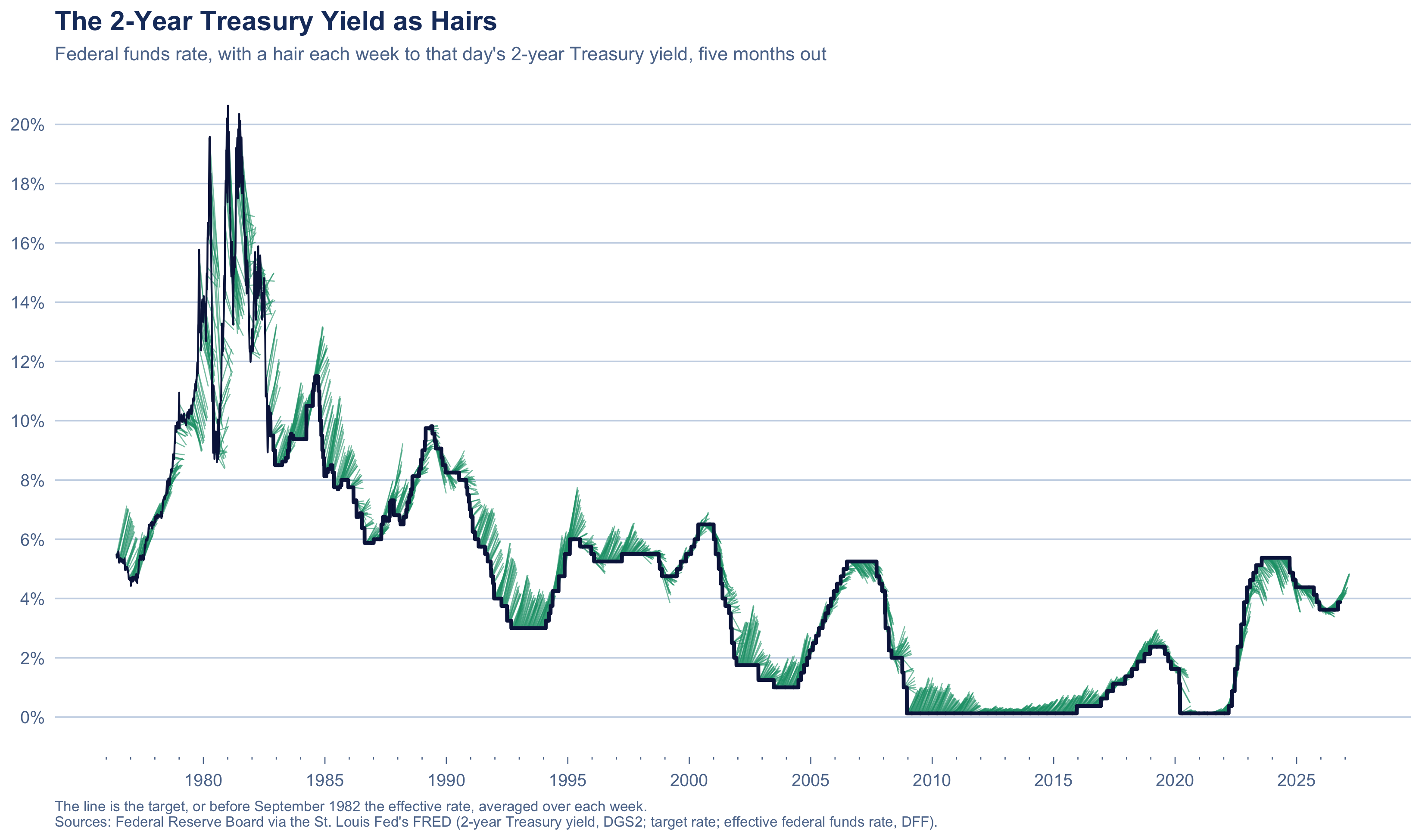
Below, we pull the data and set up these hairs. There’s a yield for every trading day, which would make a very hairy plot, so we draw one hair a week: from that day’s target rate to that day’s 2-year yield, five months out.

Source Detail: U.S. Treasury Securities at 2-Year Constant Maturity (click to expand)

The data is easily downloaded from the FRED database, series DGS2: the market yield on US Treasury securities at 2-year constant maturity, quoted on an investment basis, from the Federal Reserve Board’s H.15 release. Daily, in percent, from June 1976. The fetch_fred.py script downloads it with the other Treasury yields, and build_dataset.py writes it to data/treasury_2y.csv, dropping holidays, which have no quote.

Each trading day the Treasury fits a par yield curve to quotes on the most recently auctioned securities, and the 2-year constant maturity yield is read off that curve at exactly two years.

Each hair uses the yield on the last trading day of a week, not FRED’s weekly or monthly series (WGS2YR, GS2), which average the business days, so every hair starts on a day the yield was actually observed. It runs from the target that day to the yield, placed five months later. The hairs start with the 2-year series in June 1976 and stop at the last complete week.

Why five months? It was just a suggestion, not one chosen by testing, so in the end it is an arbitrary choice. The forecast evaluation below shows how other offsets do.

Citations.

Code

two_year <- read_csv("../data/treasury_2y.csv", show_col_types = FALSE)
# DFF has a value for every calendar day, so a seven-day mean is one week.
effective <- read_csv("../data/fed_funds_effective.csv", show_col_types = FALSE) |>
  arrange(date) |>
  mutate(week_mean = as.numeric(stats::filter(rate_pct, rep(1 / 7, 7), sides = 1)))

# This section's own color, caption and helpers, kept here so every other plot
# in the notebook renders as before.
two_year_color <- "#1B9E77"
two_year_caption <- paste(
  "Sources: Federal Reserve Board via the St. Louis Fed's FRED",
  "(2-year Treasury yield, DGS2; target rate; effective federal funds rate, DFF)."
)
offset_months <- 5

# The same day `k` months after `d`, or the month's last day if it is shorter.
months_after <- function(d, k) lubridate::add_with_rollback(d, lubridate::period(k, "months"))

# The rate on day `d`: the target, or before the target series begins, the
# effective rate's mean over the week to `d`.
policy_rate <- function(d) {
  target <- ffr$target_mid[match(d, ffr$date)]
  ifelse(is.na(target), effective$week_mean[match(d, effective$date)], target)
}

# One hair a week, from the last trading day with a quote, in the same long
# format as hairs.csv. The latest week is left out: it may not be over.
two_year_hairs <- two_year |>
  mutate(week = lubridate::floor_date(date, "week", week_start = 1)) |>
  filter(week < max(week)) |>
  group_by(week) |>
  slice_max(date, n = 1) |>
  ungroup() |>
  transmute(
    source = "two_year_offset",
    as_of = date,
    target_date = months_after(date, offset_months),
    horizon_months = offset_months,
    rate_pct
  )

# Each hair starts on the line at its forecast date, reading the line a day
# later as hair_path() does, then runs straight to its one point.
two_year_path <- function(h) {
  bind_rows(
    h |> transmute(as_of, target_date = as_of, rate_pct = policy_rate(as_of + 1)),
    h |> select(as_of, target_date, rate_pct)
  ) |>
    filter(!is.na(rate_pct))
}

# The line: the effective rate's weekly mean until the target series begins,
# then the target.
two_year_line <- bind_rows(
  effective |>
    filter(date >= min(two_year_hairs$as_of)) |>
    transmute(date, rate = week_mean, kind = "effective"),
  ffr |> transmute(date, rate = target_mid, kind = "target")
)

Code

ggplot() +
  geom_line(
    data = two_year_path(two_year_hairs), aes(target_date, rate_pct, group = as_of),
    color = two_year_color, alpha = 0.6, linewidth = 0.3, lineend = "round"
  ) +
  geom_line(data = two_year_line, aes(date, rate, linewidth = kind), color = RATE, lineend = "round") +
  scale_linewidth_manual(values = c(effective = 0.5, target = 1.0), guide = "none") +
  scale_x_years(min(two_year_line$date), max(two_year_hairs$target_date)) +
  scale_y_continuous(labels = label_number(suffix = "%"), breaks = seq(0, 20, 2)) +
  coord_cartesian(ylim = c(-0.3, NA)) +
  labs(
    title = "The 2-Year Treasury Yield as Hairs",
    subtitle = "Federal funds rate, with a hair each week to that day's 2-year Treasury yield, five months out",
    caption = paste0(
      "The line is the target, or before September 1982 the effective rate, averaged over each week.\n",
      two_year_caption
    )
  ) +
  theme_hairy()

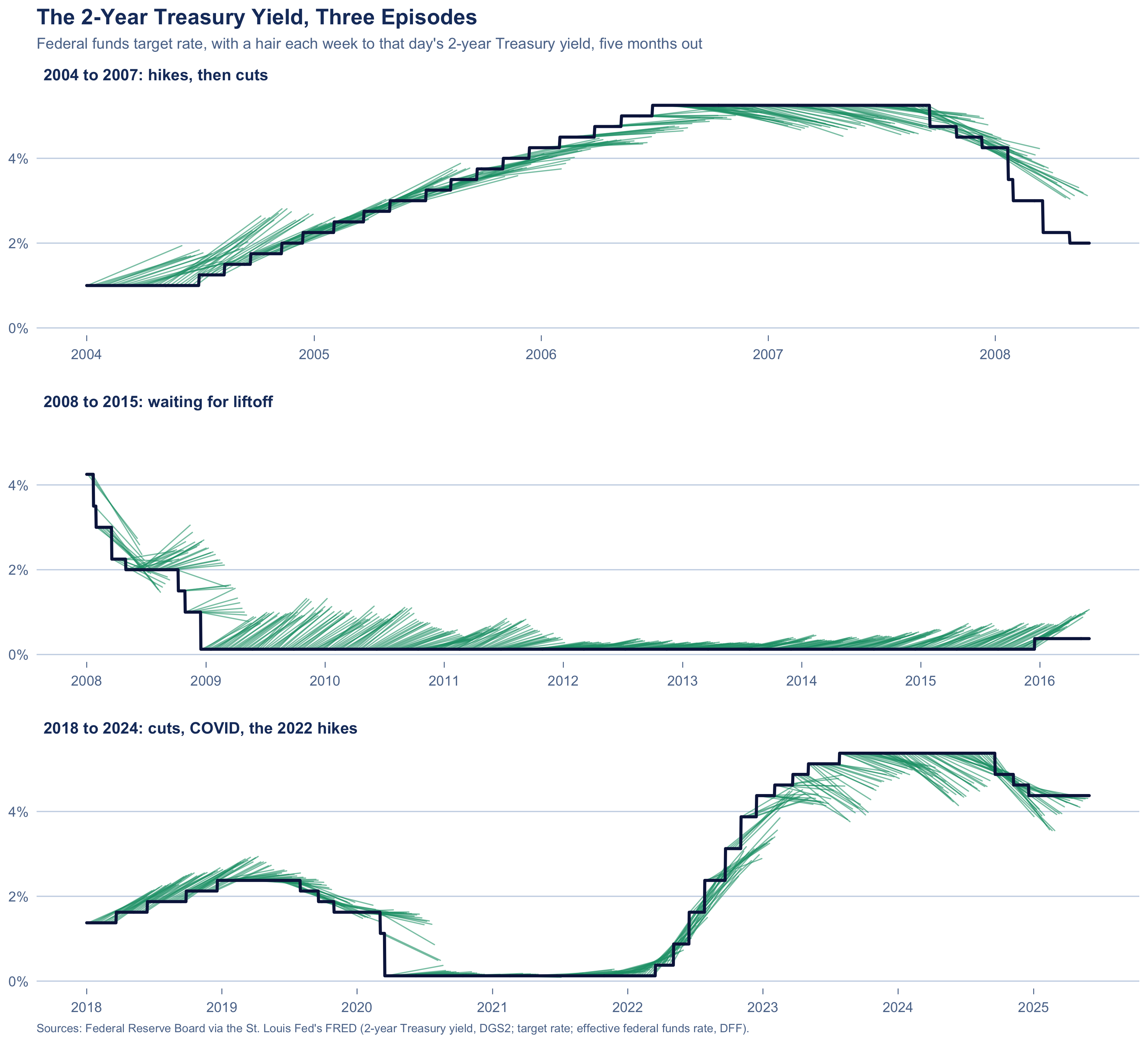
Three stretches up close: hikes then cuts, the long wait for liftoff, and cuts, COVID and the 2022 hikes.

Code

episodes <- tibble(
  episode = c(
    "2004 to 2007: hikes, then cuts",
    "2008 to 2015: waiting for liftoff",
    "2018 to 2024: cuts, COVID, the 2022 hikes"
  ),
  from = as.Date(c("2004-01-01", "2008-01-01", "2018-01-01")),
  to = as.Date(c("2007-12-31", "2015-12-31", "2024-12-31"))
) |>
  mutate(episode = factor(episode, levels = episode))

# Hairs made in each stretch, and the target out to where the last of them ends.
episode_hairs <- cross_join(episodes, two_year_path(two_year_hairs)) |>
  filter(as_of >= from, as_of <= to)
episode_rate <- cross_join(episodes, ffr) |>
  filter(date >= from, date <= months_after(to, offset_months))

ggplot() +
  geom_line(
    data = episode_hairs, aes(target_date, rate_pct, group = as_of),
    color = two_year_color, alpha = 0.6, linewidth = 0.4, lineend = "round"
  ) +
  rate_line(episode_rate) +
  facet_wrap(~episode, ncol = 1, scales = "free_x") +
  scale_x_years(as.Date("2004-01-01"), as.Date("2025-12-31"), every = 1) +
  scale_y_continuous(labels = label_number(suffix = "%")) +
  labs(
    title = "The 2-Year Treasury Yield, Three Episodes",
    subtitle = "Federal funds target rate, with a hair each week to that day's 2-year Treasury yield, five months out",
    caption = two_year_caption
  ) +
  theme_hairy() +
  theme(
    strip.text = element_text(color = INK, face = "bold", hjust = 0, size = 11),
    panel.spacing.y = unit(1.2, "lines")
  )

Forecast Evaluation for 2-Year Yields

How well does this forecast perform? Let’s check. For each hair whose end date has passed, that is, each hair whose accuracy we can check, we compare how far the target ended up from two forecasts: the 2-year Treasury yield, as a prediction for five months out, and no change, the target on the day the hair starts. Before September 1982 the effective rate stands in for the target. Errors are in percentage points, and “Hair closer” is the share of weeks where the hair’s error was the smaller of the two.

Code

two_year_check <- two_year_hairs |>
  mutate(
    known = policy_rate(as_of + 1),
    outcome = policy_rate(target_date)
  ) |>
  filter(!is.na(known), !is.na(outcome)) |>
  mutate(
    Era = cut(
      as_of,
      as.Date(c("1976-01-01", "1982-09-27", "1994-01-01", "2008-01-01", "2016-01-01", "2100-01-01")),
      labels = c("1976 to 1982, effective rate", "1982 to 1993", "1994 to 2007", "2008 to 2015", "2016 on"),
      right = FALSE
    ),
    yield_error = abs(rate_pct - outcome),
    flat_error = abs(known - outcome)
  )

error_summary <- function(d) {
  summarise(
    d,
    Weeks = n(),
    yield_abs = mean(yield_error),
    flat_abs = mean(flat_error),
    closer = mean(yield_error < flat_error)
  )
}

bind_rows(
  two_year_check |> group_by(Era) |> error_summary() |> mutate(Era = as.character(Era)),
  two_year_check |> error_summary() |> mutate(Era = "All weeks")
) |>
  gt_basic() |>
  tab_spanner("Mean absolute error", c(yield_abs, flat_abs)) |>
  cols_label(yield_abs = "2-year yield", flat_abs = "No change", closer = "Hair closer") |>
  fmt_number(c(yield_abs, flat_abs), decimals = 2) |>
  fmt_percent(closer, decimals = 0)

Era	Weeks	Mean absolute error		Hair closer
Era	Weeks	2-year yield	No change	Hair closer
1976 to 1982, effective rate	330	2.39	2.42	49%
1982 to 1993	588	1.13	0.73	32%
1994 to 2007	730	0.58	0.55	48%
2008 to 2015	418	0.50	0.15	5%
2016 on	541	0.35	0.45	50%
All weeks	2607	0.87	0.74	38%

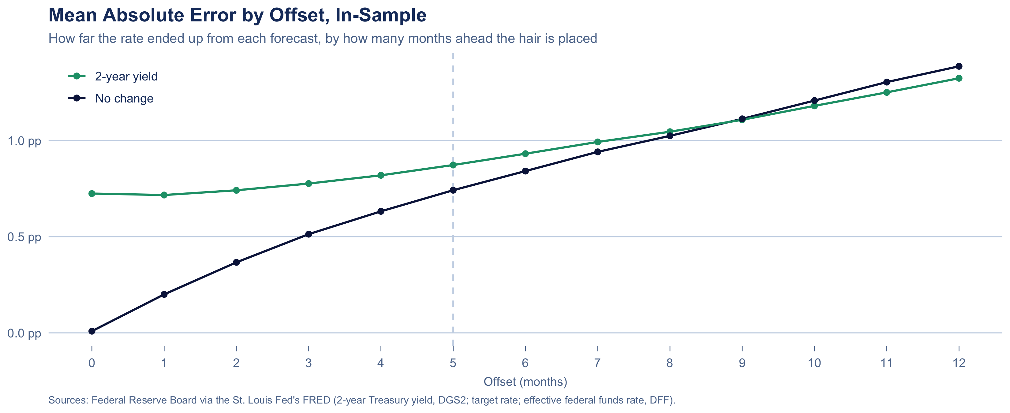
Is five months the right offset? The same errors for every offset from 0 to 12 months. This is in-sample: choosing the best offset after looking at the results flatters it.

Code

offset_errors <- lapply(0:12, function(k) {
  two_year_hairs |>
    mutate(
      known = policy_rate(as_of + 1),
      outcome = policy_rate(months_after(as_of, k))
    ) |>
    filter(!is.na(known), !is.na(outcome)) |>
    summarise(
      offset = k,
      yield = mean(abs(rate_pct - outcome)),
      flat = mean(abs(known - outcome))
    )
}) |>
  bind_rows() |>
  tidyr::pivot_longer(c(yield, flat), names_to = "forecast", values_to = "mae")

offset_labels <- c(yield = "2-year yield", flat = "No change")

ggplot(offset_errors, aes(offset, mae, color = forecast)) +
  geom_vline(xintercept = offset_months, color = GRID, linewidth = 0.6, linetype = "dashed") +
  geom_line(linewidth = 0.8) +
  geom_point(size = 1.8) +
  scale_color_manual(
    values = c(yield = two_year_color, flat = RATE), labels = offset_labels, breaks = names(offset_labels)
  ) +
  scale_x_continuous(breaks = 0:12) +
  scale_y_continuous(labels = label_number(suffix = " pp", accuracy = 0.1), limits = c(0, NA)) +
  labs(
    title = "Mean Absolute Error by Offset, In-Sample",
    subtitle = "How far the rate ended up from each forecast, by how many months ahead the hair is placed",
    x = "Offset (months)",
    caption = two_year_caption
  ) +
  theme_hairy() +
  theme(
    axis.title.x = element_text(color = INK_SOFT, size = 9.5, margin = margin(t = 6)),
    legend.position = "inside",
    legend.position.inside = c(0.01, 0.985),
    legend.justification = c(0, 1),
    legend.background = element_rect(fill = BG, color = NA)
  )

Other Sources

Other data on expected federal funds rates exist. The most direct are fed funds futures, exchange-traded contracts whose prices imply the market’s expected average federal funds rate for each coming month, and overnight index swap (OIS) curves, which do the same through swap contracts. Both price individual FOMC meetings, so their paths step rather than move smoothly, and they are the usual basis for this plot in market commentary. These series are not free (which is why they aren’t in this notebook; I couldn’t find a free copy anywhere): they require payment, through vendors such as Bloomberg, LSEG (Refinitiv), CME DataMine or Databento.

The sources above are free stand-ins for them.

The Very Hairy Plot

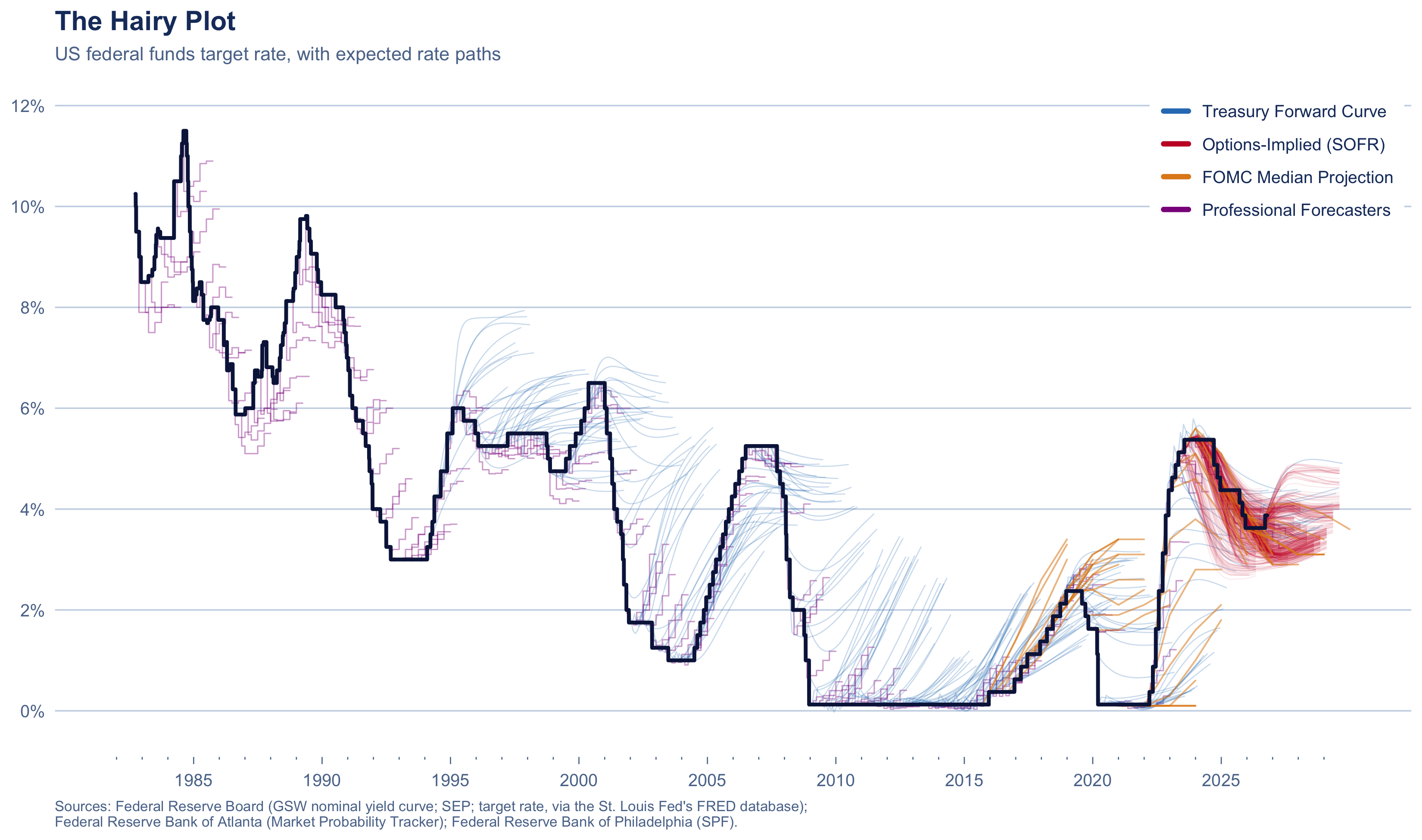
All four sources at once, against the target rate.

Code

hair_layer <- function(src, alpha, linewidth) {
  hair_geom(
    src,
    data = hair_path(hairs |> filter(source == src), src) |> mutate(source = src),
    mapping = aes(target_date, rate_pct, group = as_of, color = source),
    alpha = alpha, linewidth = linewidth, lineend = "round"
  )
}

ggplot() +
  hair_layer("spf_median", 0.40, 0.35) +
  hair_layer("treasury_forward", 0.25, 0.30) +
  hair_layer("options_implied", 0.09, 0.25) +
  hair_layer("sep_median", 0.55, 0.45) +
  rate_line(ffr) +
  scale_color_manual(
    values = pal, labels = src_label, breaks = names(pal),
    guide = guide_legend(override.aes = list(alpha = 1, linewidth = 1.4))
  ) +
  scale_x_years(as.Date("1982-01-01"), as.Date("2029-12-31")) +
  scale_y_continuous(labels = label_number(suffix = "%"), breaks = seq(0, 12, 2)) +
  coord_cartesian(
    xlim = c(as.Date("1982-01-01"), as.Date("2029-12-31")),
    ylim = c(-0.3, 12)
  ) +
  labs(
    title = "The Hairy Plot",
    subtitle = "US federal funds target rate, with expected rate paths",
    caption = paste(
      "Sources: Federal Reserve Board (GSW nominal yield curve; SEP; target rate, via the St. Louis Fed's FRED database);",
      "\nFederal Reserve Bank of Atlanta (Market Probability Tracker); Federal Reserve Bank of Philadelphia (SPF)."
    )
  ) +
  theme_hairy() +
  theme(
    legend.position = "inside",
    legend.position.inside = c(0.995, 0.985),
    legend.justification = c(1, 1),
    legend.direction = "vertical",
    legend.background = element_rect(fill = BG, color = NA),
    legend.key.spacing.y = unit(1, "pt")
  )

Forecast Evaluation

How far off each source’s forecasts were, 6 to 36 months after they were made.

Code

# Horizons scored, in months. A month is 365/12 days, so 12 months is 365 days
# and 36 months is 1,095 days: exactly where the forecasters' and Treasury
# hairs end.
horizons <- c(6, 12, 18, 24, 36)
days_ahead <- function(months) round(months * 365 / 12)

# A cell is left blank with fewer forecasts than this, or when all of them
# were made within one horizon of each other: they then all overlap, and
# there is no way to tell how much the MAE would vary.
min_n <- 8

# Every hair as it is drawn: the anchor on the target line, then the source's
# points (quarter steps for the forecasters). Where an anchor and a point share
# a date, keep the point.
paths <- lapply(names(pal), \(s) hair_path(hairs |> filter(source == s), s) |> mutate(source = s)) |>
  bind_rows() |>
  mutate(row = row_number()) |>
  group_by(source, as_of, target_date) |>
  slice_max(row, n = 1) |>
  ungroup() |>
  arrange(source, as_of, target_date)

# Read a hair at a date: straight lines between its points, or the value held
# until the next point for step sources. NA past the hair's last point, so a
# hair is never extended.
read_hair <- function(x, y, at, step) {
  approx(
    as.numeric(x), y, xout = as.numeric(at),
    method = if (step) "constant" else "linear", f = 0, rule = 1
  )$y
}

# One row per hair and horizon: the forecast, and the target on that date
# (the midpoint of the range since 2008). Only dates that have happened count.
last_day <- max(ffr$date)
scored <- paths |>
  group_by(source, as_of) |>
  reframe(
    horizon = horizons,
    about = cur_group()$as_of + days_ahead(horizons),
    forecast = read_hair(target_date, rate_pct, about, cur_group()$source %in% step_sources)
  ) |>
  filter(!is.na(forecast), about <= last_day) |>
  mutate(
    actual = ffr$target_mid[findInterval(as.numeric(about), as.numeric(ffr$date))],
    abs_error = abs(forecast - actual)
  )

Code

# Newey-West standard error of a mean. Forecasts made close together cover
# mostly the same stretch of rates, so their errors move together and the
# plain sd / sqrt(N) would be far too small. Newey-West adds the
# autocovariances up to `lag`, with Bartlett weights 1 - l / (lag + 1).
nw_se <- function(x, lag) {
  n <- length(x)
  u <- x - mean(x)
  lag <- min(lag, n - 1)
  v <- sum(u^2) / n
  for (l in seq_len(lag)) {
    v <- v + 2 * (1 - l / (lag + 1)) * sum(u[-(1:l)] * u[1:(n - l)]) / n
  }
  sqrt(v / n)
}

# The lag is how many forecasts a source makes within one horizon: two
# forecasts closer together than that overlap. Typical spacing is the median
# gap between a source's hairs (a day for options, a quarter for the SEP).
spacing <- hairs |>
  distinct(source, as_of) |>
  arrange(source, as_of) |>
  group_by(source = as.character(source)) |>
  summarise(gap = median(as.numeric(diff(as_of))))

# MAE, its standard error and N for each source and horizon, within `groups`.
summarise_errors <- function(d, ...) {
  d |>
    left_join(spacing, by = "source") |>
    arrange(as_of) |>
    group_by(source, ..., horizon) |>
    summarise(
      n = n(),
      made_over = as.numeric(max(as_of) - min(as_of)),
      mae = mean(abs_error),
      se = nw_se(abs_error, ceiling(days_ahead(first(horizon)) / first(gap))),
      .groups = "drop"
    )
}

# A cell: MAE, (SE), [N] on three lines, right-aligned in a monospaced font so
# the decimals line up. The trailing space on the MAE matches the closing
# parenthesis under it.
eval_cell <- function(mae, se, n, made_over, horizon) {
  ifelse(
    n < min_n | made_over < days_ahead(horizon), "",
    sprintf('<span class="ev">%.2f&nbsp;<br>(%.2f)<br>[%d]</span>', mae, se, n)
  )
}

# Booktabs-style rules, the source name in the body font, the numbers in the
# monospaced one.
gt_eval <- function(d, num_cols) {
  gt_basic(d) |>
    fmt_passthrough(columns = all_of(num_cols), escape = FALSE) |>
    cols_align("right", columns = all_of(num_cols)) |>
    tab_options(
      table.border.top.style = "solid", table.border.top.width = px(2), table.border.top.color = INK,
      heading.border.bottom.color = INK, column_labels.border.top.color = INK,
      column_labels.border.top.width = px(2), column_labels.border.lr.color = "transparent",
      table.border.bottom.width = px(2), table.border.bottom.color = INK,
      column_labels.border.bottom.color = INK, column_labels.border.bottom.width = px(1),
      table_body.hlines.color = "transparent", table_body.border.bottom.color = INK,
      source_notes.font.size = px(13), data_row.padding = px(8)
    ) |>
    tab_style(cell_text(whitespace = "nowrap"), cells_body(columns = Source)) |>
    opt_css(".ev { font-family: 'Courier Prime', ui-monospace, monospace; white-space: nowrap; line-height: 1.35; }")
}

se_note <- "(Newey-West standard error, which corrects for overlapping forecasts)"

# Cells for the forecasts made within each window of `windows` (columns
# `name`, `from`, `to`), one column per window.
window_cells <- function(d, windows) {
  d |>
    cross_join(windows) |>
    filter(as_of >= from, as_of <= to) |>
    summarise_errors(name) |>
    mutate(cell = eval_cell(mae, se, n, made_over, horizon)) |>
    select(source, name, cell) |>
    tidyr::pivot_wider(names_from = name, values_from = cell)
}

# One row per source, in the usual order, one column per window.
window_table <- function(cells, windows, spanner) {
  d <- tibble(source = names(pal)) |> left_join(cells, by = "source")
  for (nm in setdiff(windows$name, names(d))) d[[nm]] <- ""
  d |>
    mutate(Source = src_label[source], .keep = "unused", .before = 1) |>
    mutate(across(all_of(windows$name), \(x) tidyr::replace_na(x, ""))) |>
    select(Source, all_of(windows$name)) |>
    gt_eval(windows$name) |>
    tab_spanner(label = spanner, columns = all_of(windows$name))
}

By Horizon

Code

by_horizon <- summarise_errors(scored) |>
  mutate(cell = eval_cell(mae, se, n, made_over, horizon)) |>
  select(source, horizon, cell) |>
  tidyr::pivot_wider(names_from = horizon, values_from = cell, values_fill = "")

hairs |>
  group_by(source = as.character(source)) |>
  summarise(N = n_distinct(as_of), From = format(min(as_of), "%Y")) |>
  left_join(by_horizon, by = "source") |>
  mutate(source = factor(source, levels = names(pal))) |>
  arrange(source) |>
  mutate(Source = src_label[as.character(source)], .keep = "unused", .before = 1) |>
  mutate(across(as.character(horizons), \(x) tidyr::replace_na(x, ""))) |>
  gt_eval(as.character(horizons)) |>
  cols_align("right", columns = c(N, From)) |>
  tab_spanner(label = "Months ahead", columns = as.character(horizons)) |>
  tab_source_note(paste("Each cell: mean absolute error in percentage points,", paste0(se_note, ","), "[N forecasts scored]. N in the second column counts all of a source's hairs.")) |>
  tab_source_note("Error is the forecast at that horizon against the target rate, or the midpoint of the target range, on that date. Forecasts are read off each hair as drawn above, never past its last point.") |>
  tab_source_note("None of the sources measures the target itself: Treasury forwards include a term premium, options price SOFR, and the forecasters predict the three-month bill, so part of each error is built in.") |>
  tab_source_note(paste0("Blank: the source doesn't reach that far, or too few of its forecasts have come due (fewer than ", min_n, ", or all made within one horizon of each other)."))

Source	N	From	Months ahead
Source	N	From	6	12	18	24	36
Treasury Forward Curve	264	1994	0.37 (0.05) [260]	0.85 (0.13) [256]	1.29 (0.20) [251]	1.64 (0.25) [247]	2.11 (0.32) [239]
Options-Implied (SOFR)	893	2023	0.26 (0.04) [768]	0.44 (0.08) [644]	0.48 (0.09) [518]
FOMC Median Projection	44	2015	0.32 (0.07) [42]	0.73 (0.24) [40]	1.16 (0.38) [38]	1.61 (0.51) [36]	2.15 (0.27) [17]
Professional Forecasters	176	1982	0.53 (0.06) [174]	1.02 (0.12) [172]
Each cell: mean absolute error in percentage points, (Newey-West standard error, which corrects for overlapping forecasts), [N forecasts scored]. N in the second column counts all of a source's hairs.
Error is the forecast at that horizon against the target rate, or the midpoint of the target range, on that date. Forecasts are read off each hair as drawn above, never past its last point.
None of the sources measures the target itself: Treasury forwards include a term premium, options price SOFR, and the forecasters predict the three-month bill, so part of each error is built in.
Blank: the source doesn't reach that far, or too few of its forecasts have come due (fewer than 8, or all made within one horizon of each other).

Three Stretches

The following table limits the 12-month MAE to forecasts made in three windows: 2004 to 2007 (hikes, then cuts), 2008 to 2015 (waiting for liftoff) and 2018 to 2024 (cuts, COVID and the 2022 hikes).

Code

# The three stretches plotted in the 2-year section, by the date each
# forecast was made. Scored 12 months ahead, the
# longest horizon all four sources reach.
stretches <- tibble(
  name = c("2004 to 2007", "2008 to 2015", "2018 to 2024"),
  from = as.Date(c("2004-01-01", "2008-01-01", "2018-01-01")),
  to = as.Date(c("2007-12-31", "2015-12-31", "2024-12-31"))
)

scored |>
  filter(horizon == 12) |>
  window_cells(stretches) |>
  window_table(stretches, "12 months ahead, by year made") |>
  tab_source_note(paste("Each cell: mean absolute error in percentage points,", paste0(se_note, ","), "[N forecasts scored].")) |>
  tab_source_note(paste0("Blank: fewer than ", min_n, " forecasts from the source in that stretch."))

Source	12 months ahead, by year made
Source	2004 to 2007	2008 to 2015	2018 to 2024
Treasury Forward Curve	1.11 (0.27) [32]	0.47 (0.18) [64]	1.03 (0.27) [57]
Options-Implied (SOFR)			0.50 (0.09) [444]
FOMC Median Projection			0.97 (0.28) [27]
Professional Forecasters	1.15 (0.37) [16]	0.55 (0.20) [32]	1.08 (0.31) [28]
Each cell: mean absolute error in percentage points, (Newey-West standard error, which corrects for overlapping forecasts), [N forecasts scored].
Blank: fewer than 8 forecasts from the source in that stretch.

Common Windows

Each source covers different years, so the rows above aren’t measured over the same dates. This table limits the 12-month MAE to forecasts made since the first FOMC median projection and since the first options-implied path, so more sources share the same dates.

Code

# Windows that start where a source starts, so each later column puts one
# more source on the same dates as the rest.
first_made <- function(src) min(hairs$as_of[hairs$source == src])
common <- tibble(
  from = c(min(hairs$as_of), first_made("sep_median"), first_made("options_implied")),
  to = last_day
) |>
  mutate(name = c("All years", paste("Since", format(from[-1], "%b %Y"))))

common_note <- paste0(
  "All years: every forecast a source has. ",
  common$name[2], ": made on or after ", format(common$from[2], "%d %b %Y"),
  ", when the FOMC median projection begins. ",
  common$name[3], ": made on or after ", format(common$from[3], "%d %b %Y"),
  ", when the options-implied path begins; the only window all four sources share."
)

scored |>
  filter(horizon == 12) |>
  window_cells(common) |>
  window_table(common, "12 months ahead, by when made") |>
  tab_source_note(paste("Each cell: mean absolute error in percentage points,", paste0(se_note, ","), "[N forecasts scored].")) |>
  tab_source_note(paste(common_note, "Options-implied paths begin in March 2023, so their row is the same in every column.")) |>
  tab_source_note(paste0("Blank: the source has no forecasts in that window, or fewer than ", min_n, "."))

Source	12 months ahead, by when made
Source	All years	Since Sep 2015	Since Mar 2023
Treasury Forward Curve	0.85 (0.13) [256]	0.80 (0.22) [83]	0.41 (0.08) [21]
Options-Implied (SOFR)	0.44 (0.08) [644]	0.44 (0.08) [644]	0.44 (0.08) [644]
FOMC Median Projection	0.73 (0.24) [40]	0.73 (0.24) [40]	0.24 (0.03) [10]
Professional Forecasters	1.02 (0.12) [172]	0.82 (0.26) [40]	0.38 (0.08) [10]
Each cell: mean absolute error in percentage points, (Newey-West standard error, which corrects for overlapping forecasts), [N forecasts scored].
All years: every forecast a source has. Since Sep 2015: made on or after 17 Sep 2015, when the FOMC median projection begins. Since Mar 2023: made on or after 29 Mar 2023, when the options-implied path begins; the only window all four sources share. Options-implied paths begin in March 2023, so their row is the same in every column.
Blank: the source has no forecasts in that window, or fewer than 8.

Area Under the Curve

Rather than the miss on one date, the average gap between each hair and the target over the hair’s first 12 months: the area between the two lines, divided by 12 months. Same windows as above.

Code

# The gap between hair and target on every day from the forecast date to
# 365 days later, averaged: the area between the two lines over 12 months,
# divided by 12 months. Only hairs that reach 12 months, and whose 12 months
# have passed.
area_days <- 0:days_ahead(12)
areas <- paths |>
  group_by(source, as_of) |>
  reframe(
    date = cur_group()$as_of + area_days,
    forecast = read_hair(target_date, rate_pct, date, cur_group()$source %in% step_sources)
  ) |>
  group_by(source, as_of) |>
  filter(!anyNA(forecast), max(date) <= last_day) |>
  summarise(
    abs_error = mean(abs(forecast - ffr$target_mid[findInterval(as.numeric(date), as.numeric(ffr$date))])),
    .groups = "drop"
  ) |>
  mutate(horizon = 12)

areas |>
  window_cells(common) |>
  window_table(common, "Average gap over the first 12 months, by when made") |>
  tab_source_note(paste("Each cell: average absolute gap between hair and target over its first 12 months, in percentage points,", paste0(se_note, ","), "[N forecasts].")) |>
  tab_source_note("The gap is read every day from the forecast date to 365 days later, along the hair as drawn above; forecasts whose 12 months haven't passed are left out.") |>
  tab_source_note(paste("Windows as in the table above.", common_note)) |>
  tab_source_note(paste0("Blank: the source has no forecasts in that window, or fewer than ", min_n, "."))

Source	Average gap over the first 12 months, by when made
Source	All years	Since Sep 2015	Since Mar 2023
Treasury Forward Curve	0.40 (0.06) [256]	0.39 (0.09) [83]	0.27 (0.04) [21]
Options-Implied (SOFR)	0.25 (0.03) [644]	0.25 (0.03) [644]	0.25 (0.03) [644]
FOMC Median Projection	0.33 (0.08) [40]	0.33 (0.08) [40]	0.18 (0.02) [10]
Professional Forecasters	0.57 (0.07) [172]	0.40 (0.11) [40]	0.23 (0.02) [10]
Each cell: average absolute gap between hair and target over its first 12 months, in percentage points, (Newey-West standard error, which corrects for overlapping forecasts), [N forecasts].
The gap is read every day from the forecast date to 365 days later, along the hair as drawn above; forecasts whose 12 months haven't passed are left out.
Windows as in the table above. All years: every forecast a source has. Since Sep 2015: made on or after 17 Sep 2015, when the FOMC median projection begins. Since Mar 2023: made on or after 29 Mar 2023, when the options-implied path begins; the only window all four sources share.
Blank: the source has no forecasts in that window, or fewer than 8.

Notes

Where Does Each Hair Start?

Each hair starts on the target line at the date its forecast was made, since the rate is known then, and runs from there to the source’s first forecast; that first stretch is drawn, not forecast. A jump at the start of a hair reflects what the source measures (Treasury yields, SOFR or the three-month bill) rather than the target itself.

Session

Code

sessionInfo()

R version 4.5.2 (2025-10-31)
Platform: aarch64-apple-darwin20
Running under: macOS Sequoia 15.4.1

Matrix products: default
BLAS:   /System/Library/Frameworks/Accelerate.framework/Versions/A/Frameworks/vecLib.framework/Versions/A/libBLAS.dylib 
LAPACK: /Library/Frameworks/R.framework/Versions/4.5-arm64/Resources/lib/libRlapack.dylib;  LAPACK version 3.12.1

locale:
[1] en_US/en_US/en_US/C/en_US/en_US

time zone: America/Los_Angeles
tzcode source: internal

attached base packages:
[1] stats     graphics  grDevices utils     datasets  methods   base     

other attached packages:
[1] gt_1.3.0      scales_1.4.0  ggplot2_4.0.1 readr_2.1.5   dplyr_1.1.4  

loaded via a namespace (and not attached):
 [1] bit_4.6.0          gtable_0.3.6       jsonlite_2.0.0     crayon_1.5.3      
 [5] compiler_4.5.2     tidyselect_1.2.1   xml2_1.3.8         parallel_4.5.2    
 [9] tidyr_1.3.2        yaml_2.3.12        fastmap_1.2.0      R6_2.6.1          
[13] labeling_0.4.3     generics_0.1.3     knitr_1.51         htmlwidgets_1.6.4 
[17] tibble_3.2.1       lubridate_1.9.4    pillar_1.10.2      RColorBrewer_1.1-3
[21] tzdb_0.5.0         rlang_1.2.0        xfun_0.58          sass_0.4.10       
[25] fs_2.1.0           S7_0.2.1           bit64_4.6.0-1      timechange_0.3.0  
[29] cli_3.6.6          withr_3.0.2        magrittr_2.0.4     digest_0.6.39     
[33] grid_4.5.2         vroom_1.6.5        hms_1.1.3          lifecycle_1.0.5   
[37] vctrs_0.7.1        evaluate_1.0.5     glue_1.8.0         farver_2.1.2      
[41] purrr_1.0.4        rmarkdown_2.30     tools_4.5.2        pkgconfig_2.0.3   
[45] htmltools_0.5.9