The plot is a Lexis diagram: calendar year on x, single year of age on y, so a birth-year cohort runs as a 45-degree diagonal (age = year - birth year). The fill is the annual change in the age-specific death rate.
The data is the Human Mortality Database USA period 1x1 files, already downloaded into raw-data/hmd-mortality-data/.
Wortality-rate plots and Cause-specific plots (which need NVSS microdata) are explored in later notebooks.
Abrams L, Bramajo O, van Raalte A, Myrskylä M, Mehta NK (2026). “Insights into US life expectancy stagnation from birth cohort mortality dynamics.” PNAS 123(11), e2519356123. doi:10.1073/pnas.2519356123
How to read a Lexis diagram
The plot is a grid of cells. Each cell is one age in one calendar year, and its color is how the death rate for that age changed from the previous year.
Color. Bright Green squares are years when fewer people of that age died than the year before — mortality fell. Dark Blue squares are the opposite: more people of that age died than the year before. Pale squares in the middle are years of little change either way.
What “mortality fell” is measured against. This is worth being exact about, because it is the single easiest thing to misread. Each cell compares a group to the people who were the same age one year earlier. That’s not to the same people a year younger, and not to any long-run average. A green square at age 60 in 1995 means 60-year-olds in 1995 died at a lower rate than 60-year-olds did in 1994.
where \(m_{a,t}\) is the death rate at age \(a\) in year \(t\).
How death rates get smoothed complicates the interpretation here slightly, but we’ll get to that soon.
Columns are calendar years. Reading straight up a column tells you what happened in one particular year across every age at once. A column that is green top to bottom is a year in which death rates fell at essentially every age, which is the pattern that pushes life expectancy up. A column that is dark blue top to bottom is a bad year for everybody — an epidemic, say.
Rows are ages. Reading left to right along a row follows one age through the decades. A row that is mostly green means that being, say, 75 has been getting steadily safer year after year.
Blocks of rows matter for life expectancy. How long a 75-year-old can expect to live depends on their odds of dying at 75, at 76, at 77 and so on. So life expectancy at 75 improves when the whole band of rows from 75 upward is green, not just the single row.
Diagonals are birth cohorts. Because a square is a given age in a given year, the same group of people appears one square up and one square right in the following year. Following a diagonal therefore follows one generation as it ages. This is what the Lexis diagram is for, and it is why a feature that runs along a diagonal means something different from one that runs straight up a column.
Sign convention
The published legend runs -6% (dark blue) to +6% (bright green), and the dark features are HIV/AIDS and drug poisoning, both of which are mortality increases. So the quantity plotted is mortality improvement: the negative of the annual change in the death rate.
Log differences rather than percent changes, because that is what the paper uses (rho, multiplied by -100). At these magnitudes the two agree to within a rounding error; both are computed below.
Setup
library(tidyverse)
── Attaching core tidyverse packages ──────────────────────── tidyverse 2.0.0 ──
✔ dplyr     1.1.4     ✔ readr     2.1.5
✔ forcats   1.0.1     ✔ stringr   1.5.1
✔ ggplot2   4.0.1     ✔ tibble    3.2.1
✔ lubridate 1.9.4     ✔ tidyr     1.3.2
✔ purrr     1.0.4
── Conflicts ────────────────────────────────────────── tidyverse_conflicts() ──
✖ dplyr::filter() masks stats::filter()
✖ dplyr::lag()    masks stats::lag()
ℹ Use the conflicted package (<http://conflicted.r-lib.org/>) to force all conflicts to become errors
library(mgcv) # P-spline smoother, stands in for MortalitySmooth
Loading required package: nlme

Attaching package: 'nlme'

The following object is masked from 'package:dplyr':

    collapse

This is mgcv 1.9-3. For overview type 'help("mgcv-package")'.
library(gt) # table formatting# knitr caches each chunk independently and does not track which chunk a value# came from, so editing an upstream chunk silently leaves downstream figures# stale. autodep + dep_auto() makes it follow the variables.knitr::opts_chunk$set(autodep =TRUE)knitr::dep_auto()# Where the manually downloaded HMD files live.# Where the data is. This notebook renders in two repos, with two different# working directories, and the same layout underneath either way:## Lexis repo cwd is the project root (execute-dir: project) -> "."# website repo cwd is this page's own folder, and the ~5 MB it# reads is committed one level up, shared with the# sibling notebook page -> "../data"## Probed rather than hardcoded, because getting it wrong fails deep inside a# reader with a path that looks plausible.ROOT <-Find(\(p) dir.exists(file.path(p, "out")), c(".", "data", "../data"))if (is.null(ROOT)) stop("cannot find the data directory.\n"," Working directory is: ", getwd(), "\n"," Looked for out/ under '.', 'data' and '../data'.\n"," In the website repo, refresh the committed snapshot from the\n"," USA-mortality-Lexis-Diagram repo: python3 export_notebook_data.py",call. =FALSE)# Writing back is a Lexis-repo job: those files feed the interactive build. In# the website copy the data directory is a committed snapshot, so leave it be.WRITE_BACK <-identical(ROOT, ".")HMD_DIR <-file.path(ROOT, "raw-data/hmd-mortality-data")# The published panel covers 1981-2019, ages 25-80. HMD supplies ages 0-110+, so# starting at 25 is a crop to match the original, not a data limit. The axis is# labelled at its true lowest value so this is visible rather than implied, and# the "How wide should the age window be?" section below shows what widening it# costs and gains.AGE_FIT <-c(20, 95) # fit wider than we plot; splines are worst at their edgesAGE_PLOT <-c(25, 80)LIMIT <-6# color scale bound, percent
Data Source
The starting point is a manual download from https://mortality.org (free account required):
Log in, go to United States of America.
Under Period data, download Deaths 1x1 → Deaths_1x1.txt.
Under Period data, download Exposure-to-risk 1x1 → Exposures_1x1.txt.
Both files are fixed-width text with a two-line header. They cover 1933-2024, ages 0-110+, split Female / Male / Total.
Note the docs for country-specific data notes, and source-by-source provenance for every year. Things get nuanced, for example, US military overseas related deaths are excluded from these mortaility data from 1940-1979.
# HMD 1x1 text files share one layout, so one reader handles both.## Cleaning steps, all of them:# skip = 2 -> drop the two header lines (title line + blank line)# na = "." -> HMD writes "." for suppressed / unavailable cells# Age -> read as character because the top age is the string "110+";# strip the "+" and coerce to integer, so 110+ becomes 110# pivot -> Female/Male/Total go from three columns to a Sex column, so the# same code can produce total and sex-specific plotsread_hmd_1x1 <-function(path, value_name) { readr::read_table(path, skip =2, na =".", col_types ="icddd") |>mutate(Age =as.integer(str_remove(Age, "\\+"))) |>pivot_longer(c(Female, Male, Total), names_to ="Sex", values_to = value_name)}deaths <-read_hmd_1x1(file.path(HMD_DIR, "Deaths_1x1.txt"), "deaths")exposures <-read_hmd_1x1(file.path(HMD_DIR, "Exposures_1x1.txt"), "exposure")# Inner join on the (Year, Age, Sex) key. Both files are on the same grid, so# this is a straight merge, not a filter -- but the row count is checked.hmd <-inner_join(deaths, exposures, by =c("Year", "Age", "Sex"))stopifnot(nrow(hmd) ==nrow(deaths), nrow(hmd) ==nrow(exposures))range(hmd$Year)
[1] 1933 2024
Two things worth knowing about these numbers, neither of which is a defect:
Deaths are fractional. HMD redistributes deaths across Lexis triangles, so deaths is a real number, not a count. The Poisson fit later warns about this; the warning is suppressed and the mean estimates are unaffected.
Exposures are person-years, not headcounts, which is why mx = deaths / exposure is an occurrence-exposure rate rather than a probability.
This is explained in the docs extensively, but I think it has to do mainly with applying deaths – which usually have known ages and date of death, but without date of birth - to specific birth years. This usually requires fractionally applying deaths across multiple years.
Lexis Plot - Mortality
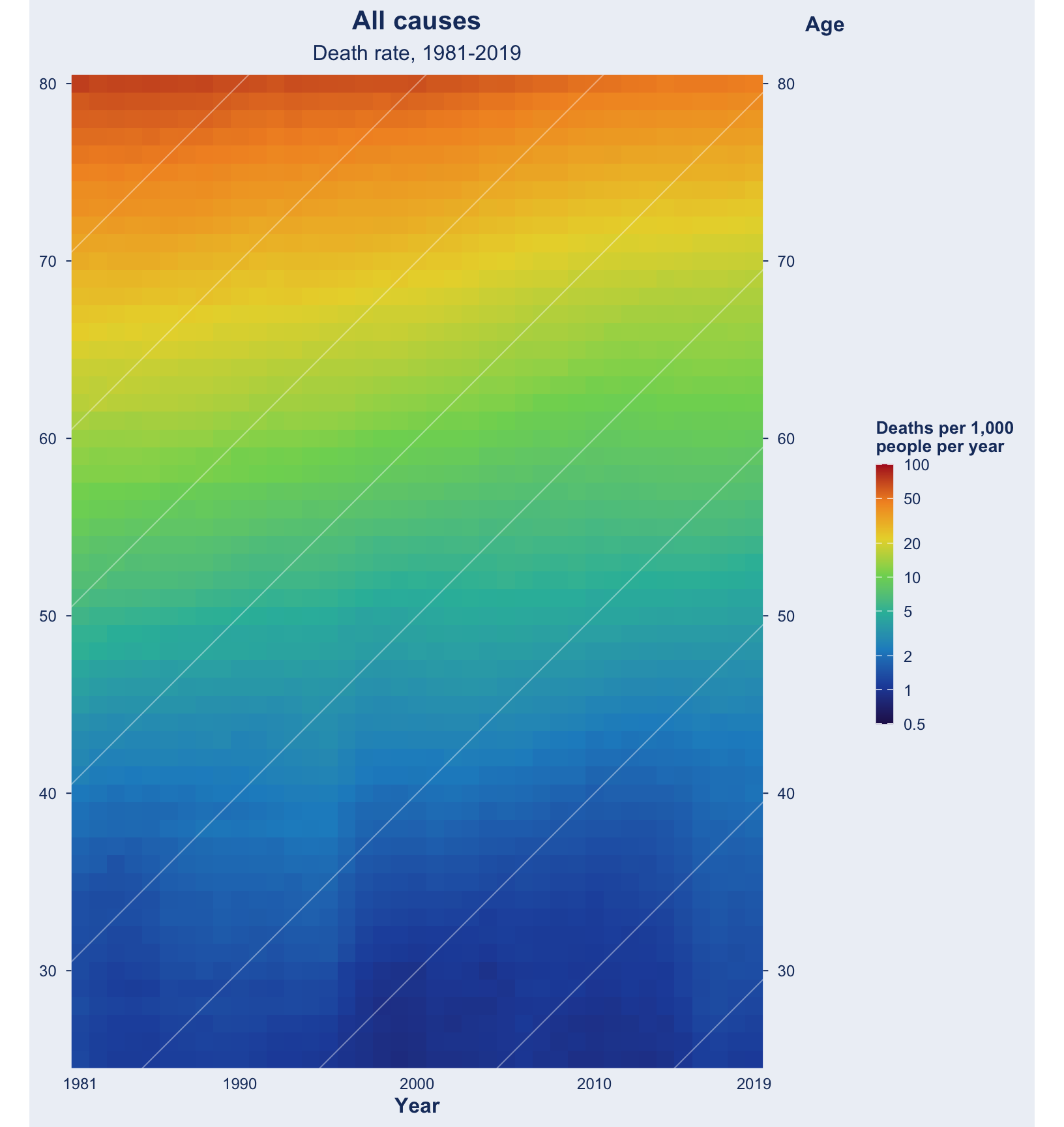
Before looking at how mortality changed, here is the level it changed from. Each cell is one age in one calendar year, colored by the death rate: the number of people of that age who died that year, per 1,000 people of that age alive.
The pattern is almost entirely vertical. Death rates climb steeply with age and that dominates everything else, which is exactly why the rest of this notebook plots the year-on-year change instead. A change plot divides that overwhelming age gradient out and leaves the part that actually moves.
The color scale is logarithmic. Over ages 25 to 80 the death rate runs from under 1 per 1,000 to over 70 per 1,000, so on a linear scale every age below about 60 would collapse into a single color.
# Same color ramp as the interactive version, cool (low) through hot (high).rate_colors <-c("#26185A", "#224EA8", "#1E8EC8", "#2CBAA8","#7ED460", "#E9D536", "#F29228", "#B01822")# Legend ticks in deaths per 1,000 per year. Round numbers spanning the plotted# range, which is about 0.86 to 73 per 1,000 over 1981-2019 at ages 25-80.rate_breaks <-c(0.5, 1, 2, 5, 10, 20, 50, 100)rates <- hmd |>filter(Sex =="Total",between(Year, 1981, 2019),between(Age, AGE_PLOT[1], AGE_PLOT[2]), exposure >0) |>mutate(per_1k =1000* deaths / exposure)ggplot(rates, aes(Year, Age, fill = per_1k)) +geom_raster() +# Cohort diagonals, faint, for orientation only.geom_abline(slope =1, intercept =-seq(1900, 1990, by =10),color ="white", alpha =0.4, linewidth =0.35) +scale_fill_gradientn(colors = rate_colors,transform ="log10",limits =c(0.5, 100),breaks = rate_breaks,labels = rate_breaks,name ="Deaths per 1,000\npeople per year",# Vertical key: with eight labelled stops the numbers need the room, and# stacking them keeps each one beside the color it belongs to.guide =guide_colourbar(barheight =unit(150, "pt"), barwidth =unit(10, "pt"),ticks.colour ="white", frame.colour =NA) ) +scale_x_continuous(expand =c(0, 0), breaks =c(1981, 1990, 2000, 2010, 2019)) +scale_y_continuous(expand =c(0, 0), position ="right",breaks =seq(30, 80, by =10),sec.axis =dup_axis(name =NULL, breaks =seq(30, 80, by =10))) +coord_fixed(1) +labs(title ="All causes", subtitle ="Death rate, 1981-2019", x ="Year", y ="Age") +theme_minimal(12) +theme(plot.background =element_rect(fill ="#EDF1F6", color =NA),panel.grid =element_blank(),axis.ticks.y =element_line(color ="#1B3A6B", linewidth =0.35),axis.ticks.length.y =unit(3, "pt"),plot.title =element_text(face ="bold", size =15, color ="#1B3A6B", hjust =0.5),plot.subtitle =element_text(size =12, color ="#1B3A6B", hjust =0.5),axis.title.x =element_text(face ="bold", color ="#1B3A6B"),axis.title.y.right =element_text(face ="bold", color ="#1B3A6B", angle =0,vjust =1.06, hjust =0, margin =margin(l =6)),axis.text =element_text(color ="#1B3A6B", size =9),legend.position ="right",legend.title =element_text(color ="#1B3A6B", size =10, face ="bold"),legend.text =element_text(color ="#1B3A6B", size =9) )
Figure 1: Death rate by age and year, all causes, sexes combined. The scale is logarithmic; cool colors are low death rates, hot colors high.
Lexis Plot - Change in Mortality
pal <-list(panel ="#EDF1F6", ink ="#1B3A6B")# The published color ramp is not linear: it fades gradually through dark blue on# the worsening side but saturates to full bright green within about two points of# zero. These stops are read off the published legend.# dark blue = mortality rose, pale = little change, bright green = mortality fellramp_values <-c(-6, -3, -1.2, 0, 0.7, 1.8, 6)ramp_colors <-c("#0B1B4A", "#2E3566", "#8C8FAE", "#F2F0EC","#B6E7D4", "#4BCCA5", "#4BCCA5")lexis_plot <-function(d, v ="improvement",title ="All causes", subtitle ="Change in mortality",cohort_by =10, label_size =3.4, label_offset =6,label_nudge =1.6, # lift text clear of its diagonallegend_width =46, # points; keep the key well short of# the panel width on tall figuresratio =1, # y:x aspect. 1 = square cells and# 45-degree cohorts. Below 1 the# panel goes landscape, which a# 91-year window needs.xbreaks =waiver(), ybreaks =waiver()) { YR <-range(d$Year); AG <-range(d$Age)# Every cohort diagonal that crosses the panel. cohorts <-seq(floor((YR[1] - AG[2]) / cohort_by) * cohort_by, YR[2] - AG[1], by = cohort_by)# Label each diagonal a few years after it enters the panel, which lines the# labels up along an anti-diagonal. label_nudge lifts the text off the line so# the rule does not strike through it. labels <-tibble(cohort = cohorts) |>mutate(enters =pmax(YR[1], cohort + AG[1]),leaves =pmin(YR[2], cohort + AG[2]),Year =pmin(enters + label_offset, leaves -3),Age = Year - cohort + label_nudge,label =if_else(cohort ==1920, "Born in 1920", as.character(cohort)) ) |>filter(leaves - enters >6, between(Age, AG[1], AG[2]))# Age ticks: default to every 10 years, always including the true lowest and# highest age on the plot so the crop is visible rather than implied.if (inherits(ybreaks, "waiver")) { ybreaks <-sort(unique(c(AG[1], seq(ceiling(AG[1] /10) *10, AG[2], 10), AG[2]))) }ggplot(d, aes(Year, Age, fill = .data[[v]])) +geom_raster() +geom_abline(slope =1, intercept =-cohorts,color ="white", alpha =0.55, linewidth =0.4) +# A cohort line has slope 1 in data units, so under coord_fixed(ratio) it# appears at atan(ratio). The labels have to follow, or they sit at 45# degrees across a line that no longer runs at 45 degrees.geom_text(data = labels, aes(Year, Age, label = label), inherit.aes =FALSE,angle =atan(ratio) *180/ pi,color ="white", size = label_size, fontface ="bold") +scale_fill_gradientn(colors = ramp_colors,values = scales::rescale(ramp_values, from =c(-LIMIT, LIMIT)),limits =c(-LIMIT, LIMIT),oob = scales::squish, # clip the extremes, as the original doesbreaks =c(-LIMIT, LIMIT),labels = \(x) paste0(x, "%"),name =NULL,guide =guide_colourbar(ticks =FALSE) ) +scale_x_continuous(expand =c(0, 0), breaks = xbreaks) +# Age ticks on both sides. sec_axis keeps them subtle -- marks only, no# gridlines, which would fight with the cohort diagonals.scale_y_continuous(expand =c(0, 0), position ="right", breaks = ybreaks,sec.axis =dup_axis(name =NULL, breaks = ybreaks)) +coord_fixed(ratio) +# at ratio 1 cohorts sit at 45 degreeslabs(title = title, subtitle = subtitle, x ="Year", y ="Age") +theme_minimal(12) +theme(plot.background =element_rect(fill = pal$panel, color =NA),panel.grid =element_blank(),axis.ticks.y =element_line(color = pal$ink, linewidth =0.35),axis.ticks.length.y =unit(3, "pt"),plot.title =element_text(face ="bold", size =15, color = pal$ink, hjust =0.5),plot.subtitle =element_text(size =12, color = pal$ink, hjust =0.5),axis.title.x =element_text(face ="bold", color = pal$ink),axis.title.y.right =element_text(face ="bold", color = pal$ink, angle =0,vjust =1.06, hjust =0, margin =margin(l =6)),axis.text =element_text(color = pal$ink, size =9),legend.position ="top",legend.key.width =unit(legend_width, "pt"),legend.key.height =unit(8, "pt"),legend.text =element_text(color = pal$ink, size =10) )}
Raw annual change, pre-smoothing
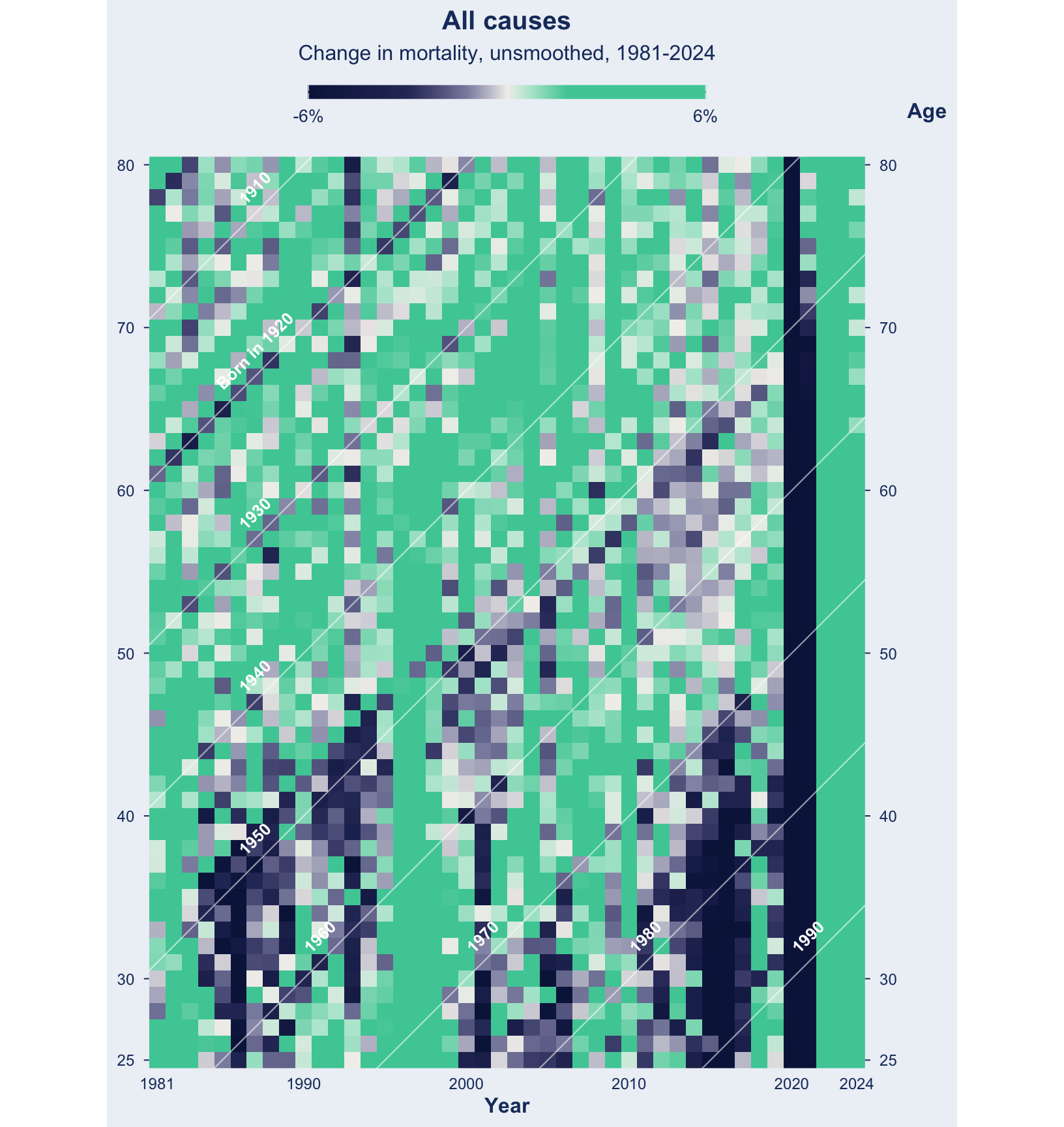
This is the plot with no model in it at all: death rate at each age, divided by the death rate at that age the year before. Exactly reproducible from the two input files, and it is the honest starting point — everything after this adds a smoother.
raw <- hmd |>filter(Sex =="Total", between(Age, AGE_PLOT[1], AGE_PLOT[2]), exposure >0) |>mutate(mx = deaths / exposure) |>arrange(Age, Year) |>group_by(Age) |># compare across years at fixed agemutate(improvement_raw =-100* (log(mx) -lag(log(mx)))) |>ungroup() |>filter(!is.na(improvement_raw), Year >=1981) |>mutate(cohort = Year - Age)
lexis_plot(raw, v ="improvement_raw",subtitle ="Change in mortality, unsmoothed, 1981-2024",xbreaks =c(1981, 1990, 2000, 2010, 2020, 2024))
Figure 2: Raw annual change in the death rate, all causes, sexes combined, no smoothing. Bright green means the rate fell against the same age the year before.
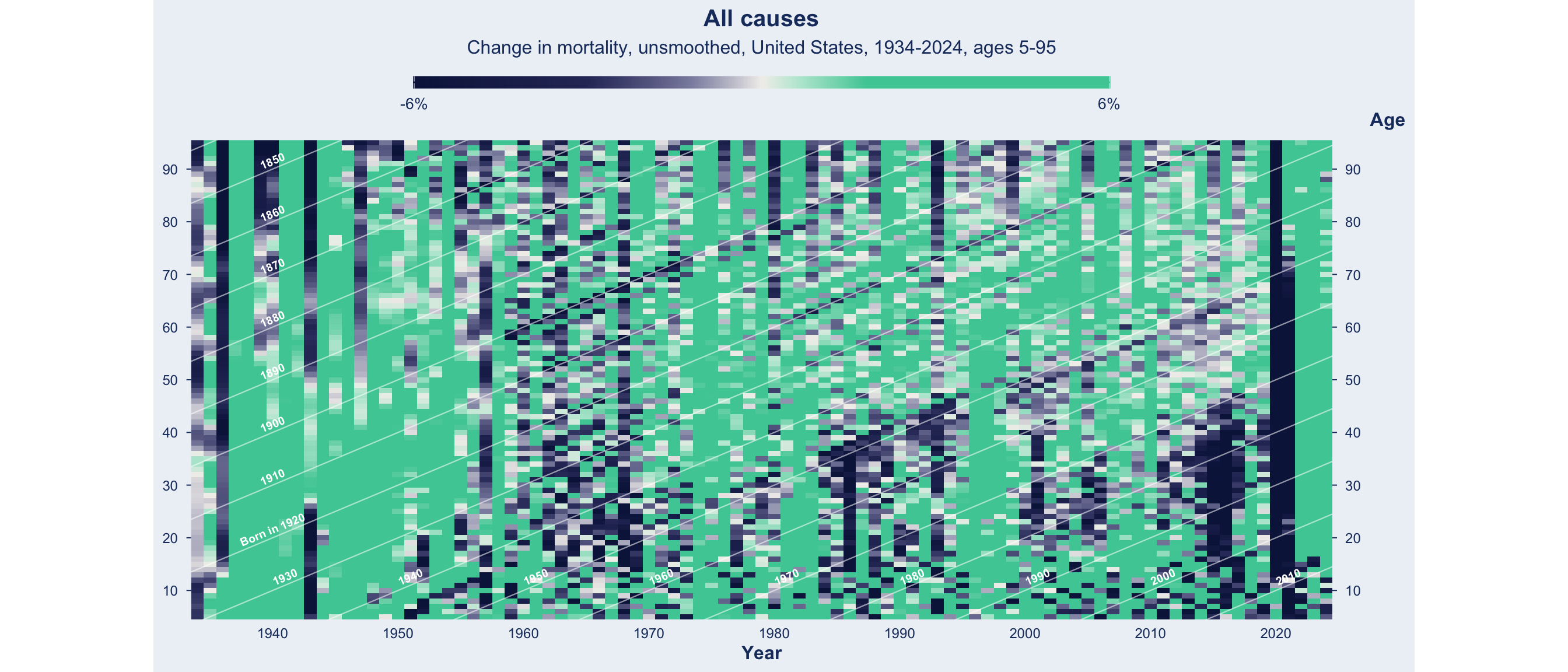
The three features the paper is about are already visible here, along with the 2020 pandemic column, which is the darkest thing on the plot by a wide margin. The cost of the raw version is noise: single-year wobble at every age makes the shapes hard to delimit, which is why the published figure is smoothed.
What is the smoother doing?
The tldr wording I settled on for figure notes:
The annual change in the age-specific death rate: -100 × (log m[a,t] − log m[a,t-1]), where m[a,t] is deaths divided by person-years of exposure at age a in year t. Smoothed values come from a 2-D P-spline (mgcv::bam, tensor-product Poisson), standing in for the deprecated MortalitySmooth package (well, it seems to be still good, but it’s archived on CRAN) used by Abrams et al. (2026). Raw values are the plain year-on-year log difference and involve no model.
Raw differences the observed rates: the death rate at an age, against the death rate at that same age the year before. No model is involved and the result is reproducible from the input files alone.
Smoothed fits one two-dimensional surface to the death counts across all ages and years at once, then differences the fitted rates. The smoothing is applied to the death rates, not to the annual changes.
Three properties of that fit:
It is not a moving average. There is no window width and no number of years being averaged. Smoothness comes from a penalty on how sharply the fitted surface is allowed to bend.
It smooths across ages as well as years.te(Year, Age) is a single basis spanning both dimensions, so the fitted rate at age 50 in 1995 draws on neighbouring calendar years and on ages either side of 50.
The amount of smoothing is estimated, not specified. We set only the basis size, which fixes the finest detail the surface is capable of showing. method = "fREML" then estimates how much of that detail to keep.
The basis used here is about one spline function per 5 calendar years, and one per 2 to 5 years of age.
Two consequences:
The age basis has to be finer than the year basis when the window includes childhood. Mortality drops sharply between age 0 and age 10, and a coarser basis smooths straight through it. build_surface below doubles the age basis when the window reaches below 15.
Smoothing spreads a single-year shock into its neighbours. 2020 bleeds visibly into 2019 and 2021. Use raw when the timing matters and smoothed when the shape does.
Build the smoothed rate surface
Abrams et al. (2026) smooth with MortalitySmooth::Mort2Dsmooth, which is archived on CRAN (essentially deprecated). This notebook uses mgcv::bam instead: a tensor-product P-spline fitted by Poisson likelihood with log exposure as an offset, which is the same method.
# Returns one tidy Lexis grid: raw rates, smoothed rates, and both versions of# the annual change.## sex : "Total", "Female" or "Male"# years : c(first, last). One year is consumed by the lag, so the first# *plotted* year is years[1] + 1.build_surface <-function(sex ="Total", years,ages_fit = AGE_FIT, ages_plot = AGE_PLOT) { m <- hmd |>filter( Sex == sex,between(Year, years[1], years[2]),between(Age, ages_fit[1], ages_fit[2]), exposure >0, # drop cells with no one at risk (none in this window)!is.na(deaths) ) |>mutate(mx = deaths / exposure)# The smoother assumes a complete rectangular year x age grid.stopifnot(nrow(m) ==n_distinct(m$Year) *n_distinct(m$Age))# --- smoothing -----------------------------------------------------------# The paper uses 2D P-splines on Poisson death counts (Camarda's# MortalitySmooth::Mort2Dsmooth, archived on CRAN). mgcv::bam() with a tensor# product P-spline basis is the maintained equivalent: same likelihood, same# penalty family, different smoothing-parameter selection (fREML vs BIC).# These should be equivolent...## Basis size follows Mort2Dsmooth's default of one knot per 5 data points,# which is what keeps the fit as smooth as the published figure. Setting k# much higher makes the smoother chase single bad years and the plot breaks# into vertical stripes.## Exception: the age basis is doubled when the window reaches below 15. The# fall in mortality from age 0 to age 10 is sharp, and a one-knot-per-5 basis# smooths straight through it -- measured as RMSE of fitted vs observed log# rate at ages 0-10, it is roughly 0.35 at k/5 against 0.08 at k/2.5. age_div <-if (ages_fit[1] <15) 2.5else5 k_year <-max(6, round(n_distinct(m$Year) /5) +3) k_age <-max(6, round(n_distinct(m$Age) / age_div) +3) fit <-withCallingHandlers(bam( deaths ~te(Year, Age, bs ="ps", k =c(k_year, k_age)) +offset(log(exposure)),family =poisson(), data = m, method ="fREML", discrete =TRUE ),# HMD deaths are fractional; the Poisson mean estimates are unaffected.warning =function(w) {if (grepl("non-integer", conditionMessage(w))) invokeRestart("muffleWarning") } )# --- annual change ------------------------------------------------------- m |>mutate(log_mx_hat =as.numeric(predict(fit, type ="link")) -log(exposure)) |>arrange(Age, Year) |>group_by(Age) |># compare across years at fixed agemutate(improvement =-100* (log_mx_hat -lag(log_mx_hat)), # smoothedimprovement_raw =-100* (log(mx) -lag(log(mx))), # unsmoothedpct_change =100* (exp(log_mx_hat) /lag(exp(log_mx_hat)) -1) ) |>ungroup() |>filter(between(Age, ages_plot[1], ages_plot[2]), !is.na(improvement)) |>mutate(cohort = Year - Age)}
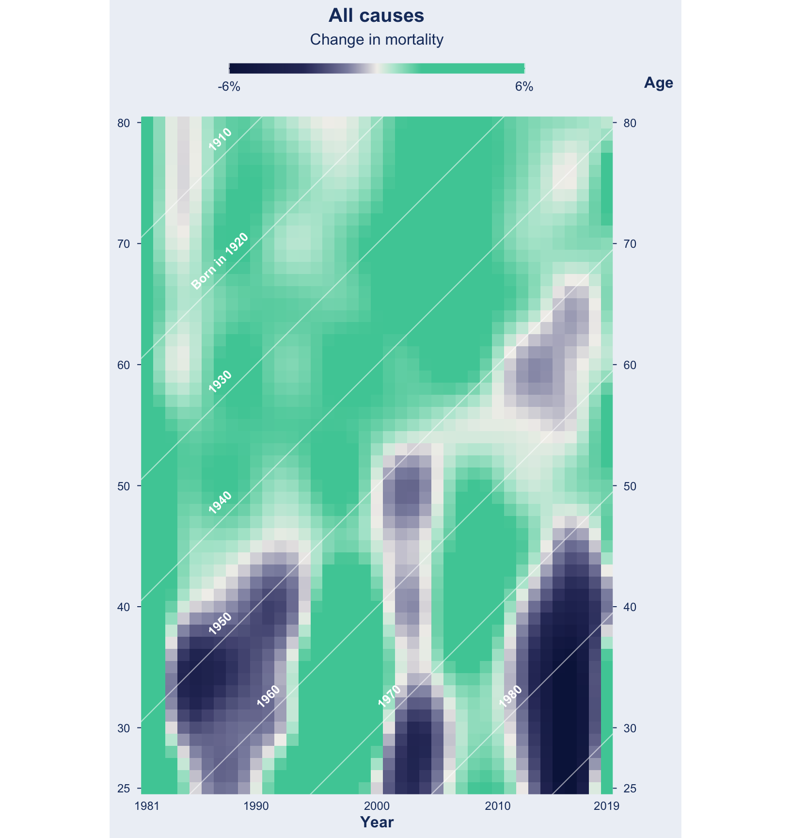
Figure 3: Annual mortality improvement, all causes, sexes combined. Bright green means the death rate fell against the same age the year before. Compare with The Economist, 17 July 2026.
Expanding Years - Going back to 1933 and up to 2024
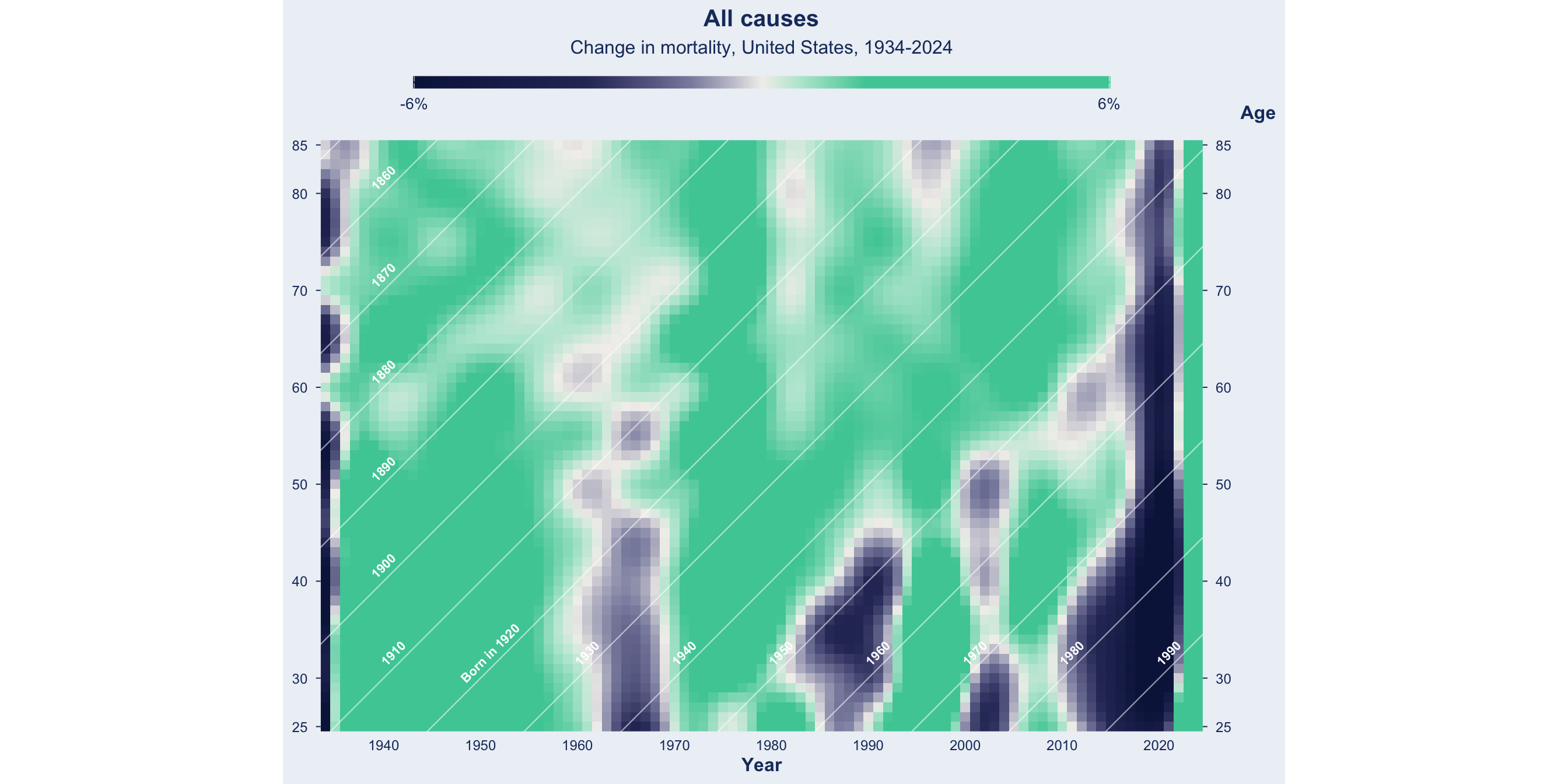
Same code, wider time window. HMD USA starts in 1933, when the death registration area first covered all states, and now runs to 2024. The panel is 91 years wide against 61 ages, so it is landscape rather than portrait.
full <-build_surface("Total", years =c(1933, 2024), ages_plot =c(25, 85))lexis_plot(full,subtitle ="Change in mortality, United States, 1934-2024",label_size =2.9,legend_width =90, # wide panel, so the key can be wider tooxbreaks =seq(1940, 2020, 10))
Figure 4: Annual mortality improvement, all causes, 1934-2024. Same color scale, clipped at plus or minus 6 percent.
What the longer window adds:
Very large improvements at young adult ages through the 1930s and 1940s. The magnitude is in the data; attributing it to any particular cause is beyond what these two files can support, so no attribution is offered here.
The 2020 pandemic.
I’m not totally sure why the Economist limited the dates from 1981 to 2019. I suspect up to 1979, mortality rate methods changes substantially, making comparisions imperfect.
1940-1979, Removal of Overseas Military Personal, and Their Deaths
Where is Vietnam, Korean and the Second World Wars?
Stated in the data notes, overseas US military related deaths were excluded from these data from 1940 to 1979. You can actually see this in the data as a significant drop in the number of 18-25 years old men in the exposure dataset, as thousands of individuals entered the military overseas, with their deaths ignored by these mortality data.
World War 2
hmd |>filter(Sex =="Male", between(Age, 16, 30), between(Year, 1940, 1946), exposure >0) |>mutate(mx = deaths / exposure) |>arrange(Age, Year) |>group_by(Age) |>mutate(improvement =-100* (log(mx) -lag(log(mx)))) |>ungroup() |>mutate(band =cut(Age, c(15, 19, 24, 30),labels =c("ages 16-19", "ages 20-24", "ages 25-30"))) |>group_by(band,Year) |>mutate(ex =sum(exposure)) |>ungroup() |>summarise(mean_improvement =round(mean(improvement, na.rm =TRUE), 1),.by =c(Year, band, ex) ) |>pivot_wider(names_from = band, values_from =c(mean_improvement,ex)) |>arrange(Year) |>select( Year ,chg_a =`mean_improvement_ages 16-19`, exp_a =`ex_ages 16-19`,chg_b =`mean_improvement_ages 20-24`, exp_b =`ex_ages 20-24`,chg_c =`mean_improvement_ages 25-30`, exp_c =`ex_ages 25-30` ) |># 1940 is the first year in the window, so it has no prior year to compare# against and every change is NaN. The row is kept for its exposure counts,# which are the pre-war baseline, but the empty changes are blanked.mutate(across(c(chg_a, chg_b, chg_c), \(x) if_else(is.nan(x), NA_real_, x))) |># Seven columns of long headers overflow the page as a plain data frame. Two# sub-columns under one spanner per age band fits, and pairs each change with# the population it was computed from.gt(rowname_col ="Year") |>tab_spanner("Ages 16-19", c(chg_a, exp_a)) |>tab_spanner("Ages 20-24", c(chg_b, exp_b)) |>tab_spanner("Ages 25-30", c(chg_c, exp_c)) |>cols_label(chg_a ="Mortality Change", exp_a ="Men",chg_b ="Mortality Change", exp_b ="Men",chg_c ="Mortality Change", exp_c ="Men") |>fmt_number(columns =c(chg_a, chg_b, chg_c), decimals =1, pattern ="{x}%") |>fmt_number(columns =c(exp_a, exp_b, exp_c), decimals =0, use_seps =TRUE) |>sub_missing(columns =c(chg_a, chg_b, chg_c), missing_text ="") |>tab_style(style =cell_text(weight ="bold"),locations =cells_column_spanners()) |># Mark the years mortality worsened. The NA guard matters: without it the 1940# row's missing changes make the condition NA rather than FALSE.tab_style(style =cell_text(color ="#C8102E"),locations =cells_body(columns =c(chg_a, chg_b, chg_c),rows = (!is.na(chg_a) & chg_a <0) | (!is.na(chg_b) & chg_b <0) | (!is.na(chg_c) & chg_c <0))) |>tab_options(table.font.size =px(13), data_row.padding =px(3),table.width =pct(100))
Ages 16-19
Ages 20-24
Ages 25-30
Mortality Change
Men
Mortality Change
Men
Mortality Change
Men
1940
4,920,994
5,701,501
6,504,196
1941
−2.2%
4,881,094
−1.5%
5,681,972
1.7%
6,499,962
1942
5.1%
4,739,947
−2.5%
5,462,076
3.4%
6,369,912
1943
−11.8%
4,454,693
−19.9%
4,880,993
−2.7%
6,002,127
1944
−2.3%
4,106,479
−6.5%
4,060,168
1.3%
5,378,512
1945
3.1%
3,932,925
15.4%
4,017,852
3.1%
5,384,575
1946
12.7%
4,042,658
14.4%
4,976,411
12.0%
6,315,446
Note that in 1943, male mortality fell by about 20% among ages 20–24 and 12% among ages 16–19, compared with only about 3% among ages 25–30. Mortality was again lower in 1944, before swinging sharply positive in 1945–46 as the war ended.
You can also see the number of exposures (labeled “Men”) decline dramatically as these individuals entered the military, traveled overseas, and were removed from the exposures and deaths dataset.
This removal also complicates the interpretation of other mortality statistics. Removing these men reduces the denominator used to calculate death rates for the remaining U.S. population. More importantly, military service is unlikely to be randomly distributed across the population, so their removal may be correlated with particular causes of mortality. As a result, changes in observed death rates may partly reflect changes in who remains in the population at risk, rather than changes in mortality risk alone.
full_wide <- hmd |>filter(Sex =="Total", between(Age, 5, 95), exposure >0) |>mutate(mx = deaths / exposure) |>arrange(Age, Year) |>group_by(Age) |>mutate(improvement_raw =-100* (log(mx) -lag(log(mx)))) |>ungroup() |>filter(!is.na(improvement_raw)) |>mutate(cohort = Year - Age)# 91 years by 91 ages is a square panel at ratio 1, which is why this figure kept# coming out square no matter what fig-width said. ratio 0.42 squashes the age# axis so the panel fills a landscape figure.lexis_plot(full_wide, v ="improvement_raw",subtitle ="Change in mortality, unsmoothed, United States, 1934-2024, ages 5-95",label_size =2.6,legend_width =90,ratio =0.42,xbreaks =seq(1940, 2020, 10),ybreaks =seq(10, 90, 10))
Figure 5: Raw annual change, all causes, 1934-2024, ages 5-95, unsmoothed. Widening the age window brings in the 1943 war column at ages 18-25, which the 25-80 crop removes entirely.
For the same window smoothed — which is the better view of the slow features and the worse view of the sharp ones — see the 1934-2024 plot earlier in this section.
COVID
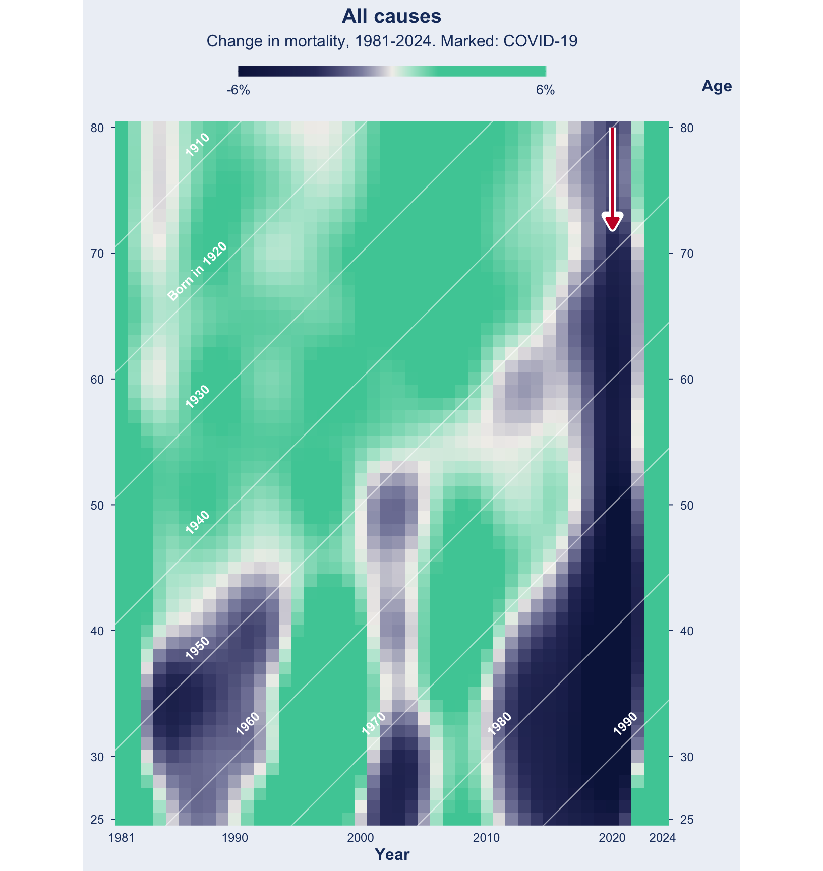
COVID-19, starting in 2020, is a vertical stripe striking every generation in the same year, with dramatic improvements following the release of vaccines and broad immunity.
2020 is about -18% worsening of mortality averaged over ages 25-85, three times worse than any other year in the modern record, and 2021 is a further -8%. 2022-2024 are the rebound improvement. Note that the rebound is measured against the pandemic years, so a large positive here means “back toward normal”, not “better than 2019”.
The color scale, clipped at ±6% to match the orginal The Economist’s data visulization, cannot represent 2020 well. It is drawn at full dark blue and the true depth is three times off the end of the legend.
Annotated Mortality Events
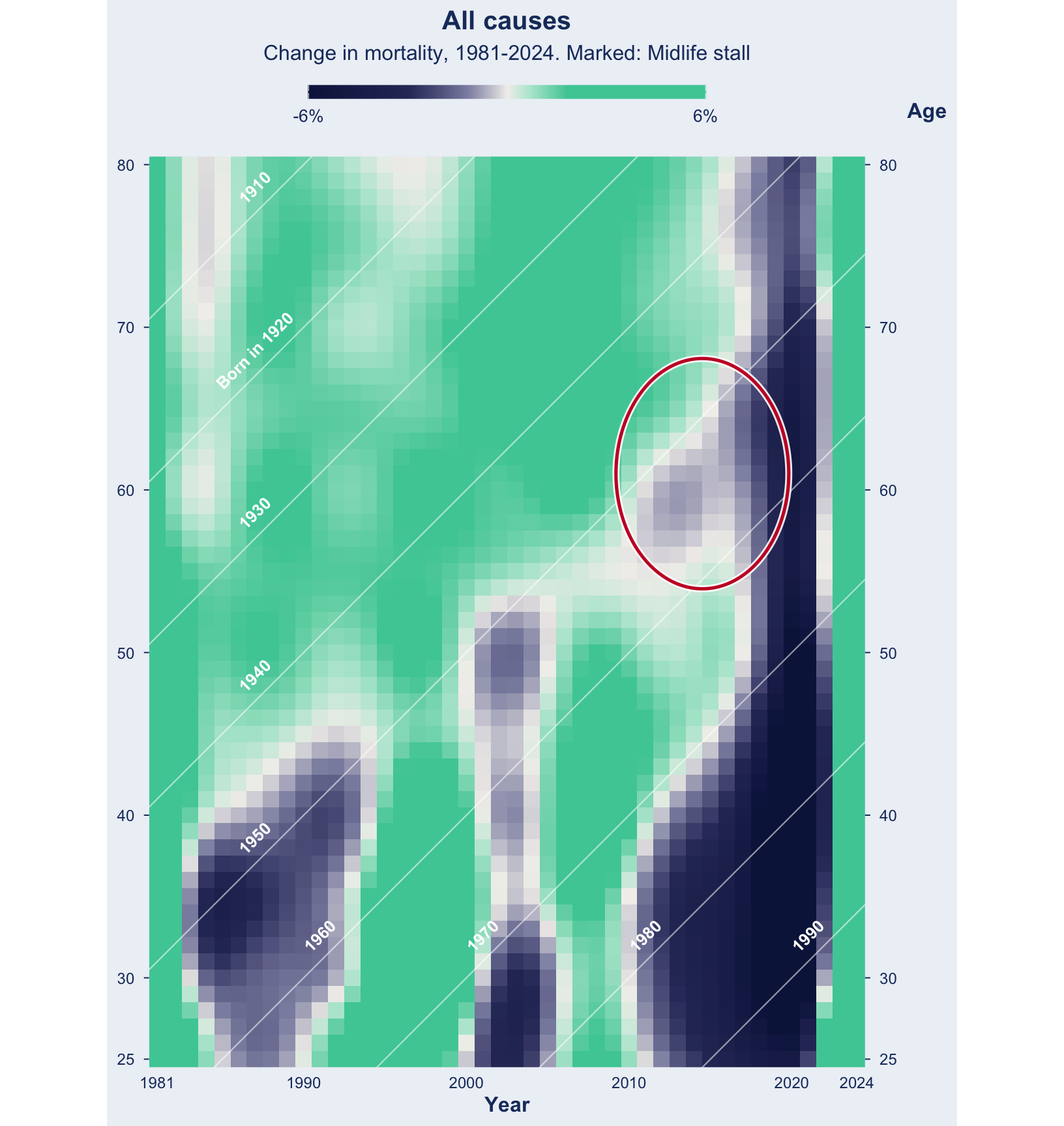
Five features stand out, all of them either mortality increases or stalls. Each tab below circles one of them on the same plot. The window runs to 2024 so that COVID is included, which means the 2020 column dominates the color scale; the earlier features read more clearly on the 1981-2019 plot above.
annotated <-build_surface("Total", years =c(1980, 2024))# Regions to circle, as c(first year, last year, lowest age, highest age).# A feature can need more than one ring, which is why each entry is a list.# COVID is the exception: it spans every age in one or two years, so a ring# round it is a tall thin sliver that reads as a scratch on the plot. It gets an# arrow from the top instead.EVENTS <-list("HIV/AIDS"=list(kind ="ellipse", regions =list(c(1980, 1993, 30, 45))),"Prescription opioids"=list(kind ="ellipse", regions =list(c(1999, 2006, 25, 35), c(1999, 2006, 45, 52))),"Fentanyl"=list(kind ="ellipse", regions =list(c(2011, 2019, 25, 45))),"Midlife stall"=list(kind ="ellipse", regions =list(c(2010, 2019, 55, 67))),"COVID-19"=list(kind ="arrow", at =2020))# An ellipse as a path, since ggforce is not a dependency here. pad leaves a# little air between the ring and the region it encloses.ellipse_path <-function(x0, x1, y0, y1, pad =1.18, n =160) { t <-seq(0, 2* pi, length.out = n)data.frame(x = (x0 + x1) /2+ (x1 - x0) /2* pad *cos(t),y = (y0 + y1) /2+ (y1 - y0) /2* pad *sin(t))}# Every mark is drawn twice, a white casing under a red line, so it stays# legible over both the dark blue and the bright green ends of the scale.annotate_event <-function(p, ev, d) {if (identical(ev$kind, "arrow")) { top <-max(d$Age) tip <- top -8for (yr in ev$at) { p <- p +annotate("segment", x = yr, xend = yr, y = top, yend = tip,color ="white", linewidth =2.6,arrow =arrow(length =unit(11, "pt"), type ="closed")) +annotate("segment", x = yr, xend = yr, y = top, yend = tip,color ="#C8102E", linewidth =1.2,arrow =arrow(length =unit(8, "pt"), type ="closed")) }return(p) }for (r in ev$regions) { e <-ellipse_path(r[1], r[2], r[3], r[4]) p <- p +annotate("path", x = e$x, y = e$y, color ="white", linewidth =1.9, alpha =0.9) +annotate("path", x = e$x, y = e$y, color ="#C8102E", linewidth =0.9) } p}
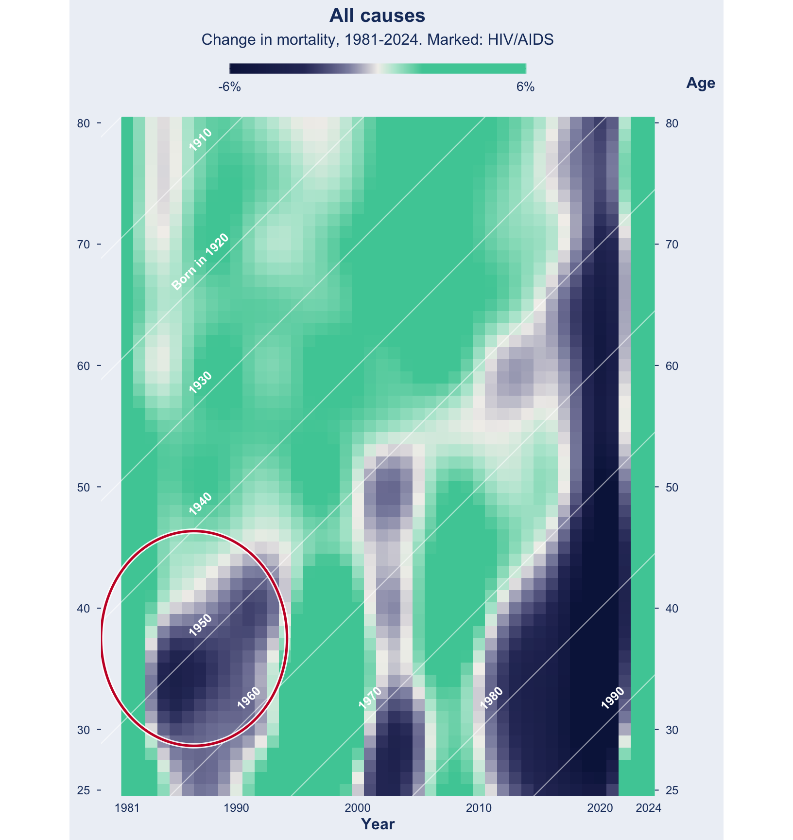
Tab 1. Ages ~30-45, 1980-1993, HIV/AIDS. Death rates at these ages rose year on year for most of a decade.
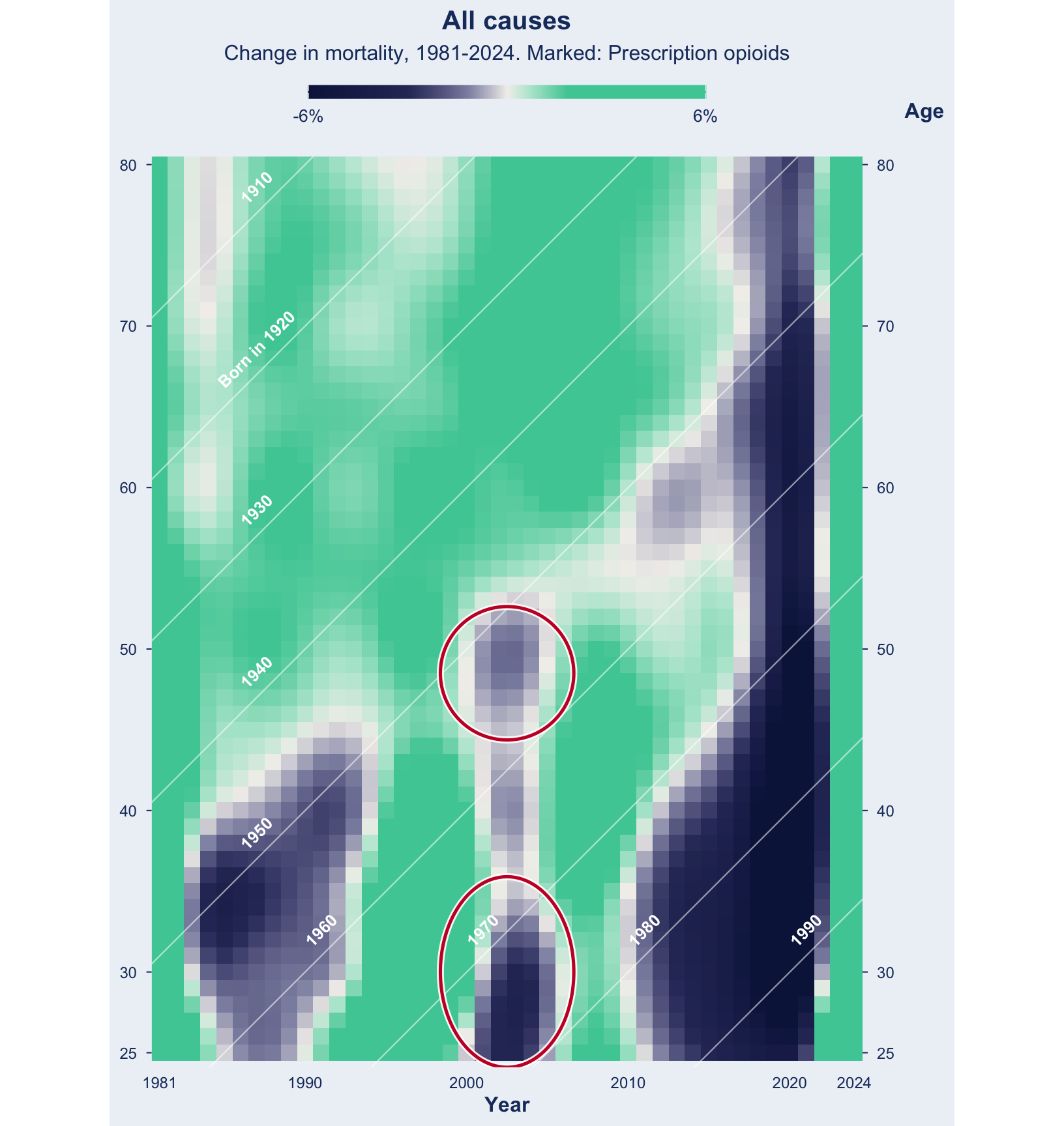
Tab 2. Ages ~25-35 and ~45-52, 1999-2006, the early prescription-opioid era. Narrower and weaker than the other two.
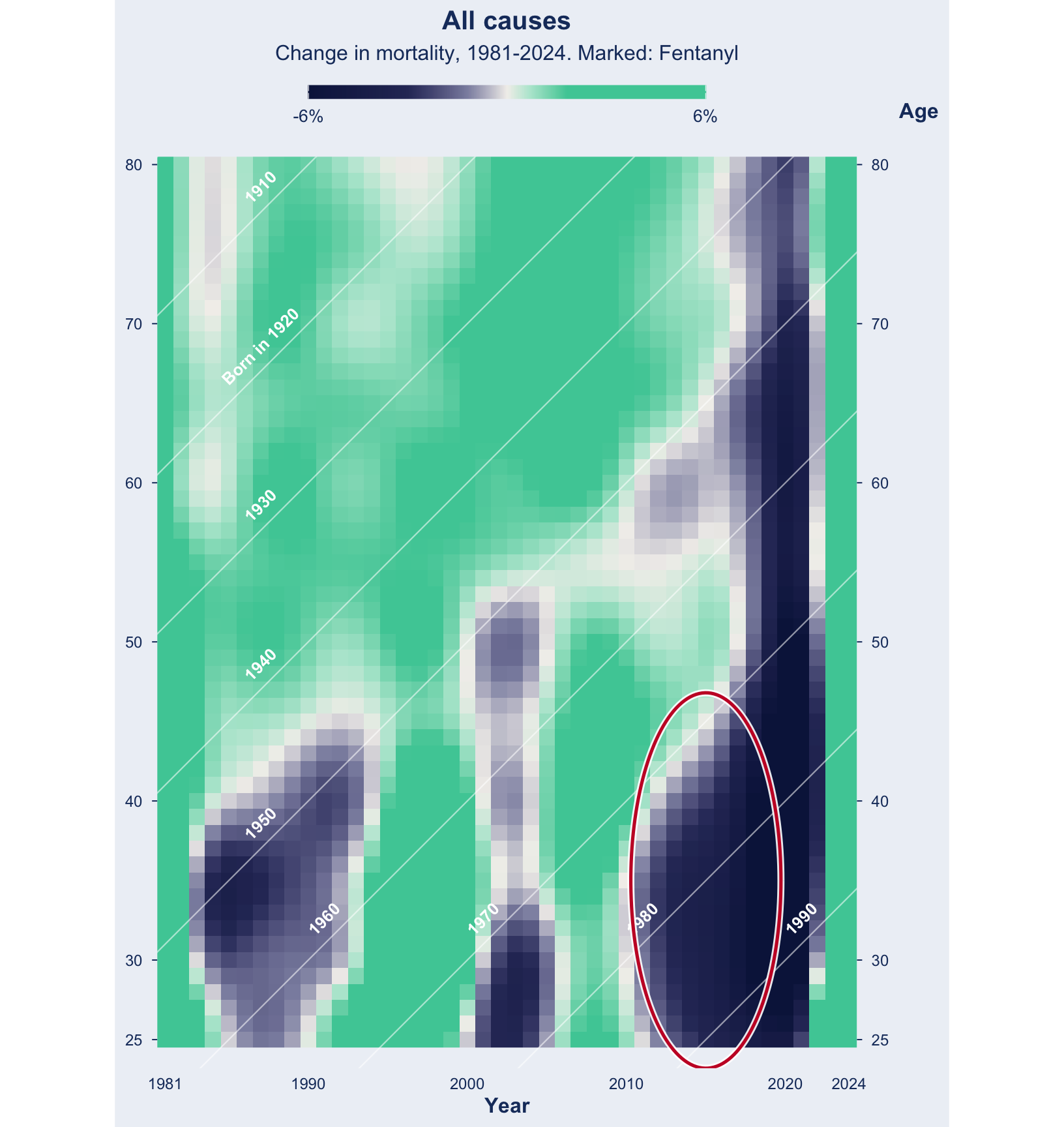
Tab 3. Ages ~25-45, 2011-2019, the fentanyl era. The strongest worsening anywhere on the plot.
Tab 4. Ages ~55-67, 2010 onward, the midlife cohort feature the paper is built around. This one is easy to miss, because it is not a period of rising mortality. It is a region where mortality simply stopped improving: the annual change sits at roughly zero. That matters because everywhere else on the plot, and in particular ages 70-80 over the same years, mortality kept falling at over 1% a year. When you zoom into cause-specific mortality, you see cardiovascular disease related mortality among this age group and year range worsen.
Tab 5. All adult ages, 2020-2021, COVID-19. Unlike the other four, this one is a vertical stripe rather than a band or a diagonal: it strikes every age in the same two years, then reverses.
Everything above reads two text files from disk. These are the alternatives, none of which changes the numbers.
HMDHFDplus — the same HMD files over the API
The maintained R client for mortality.org. Not installed here; the manual download above is one fewer moving part and leaves an auditable file on disk.
install.packages("HMDHFDplus")library(HMDHFDplus)# Credentials belong in ~/.Renviron as HMD_USER / HMD_PASS, not in this file.deaths <-readHMDweb("USA", "Deaths_1x1", Sys.getenv("HMD_USER"), Sys.getenv("HMD_PASS"))exposures <-readHMDweb("USA", "Exposures_1x1", Sys.getenv("HMD_USER"), Sys.getenv("HMD_PASS"))
HMDHFDplus::readHMD() also parses a file already on disk, and handles the 110+ age string for you:
demography::hmd.mx("USA", user, pass) returns rates and exposures as a demogdata object. Useful if you want Lee-Carter or lifetable functions on top; overkill for a Lexis diagram.
Only the first pattern is easy to find, and an earlier version of this project concluded from it that the mirror stopped at 2018. It does not. Everything is downloaded into raw-data/nber-mortality-data/ by the fetch script there.
Denominators still come from HMD exposures, as above.
CDC WONDER
https://wonder.cdc.gov/ serves the same underlying deaths as pre-tabulated counts by age, year and cause, which avoids the microdata download entirely. It is what the paper uses for its COVID-era supplement. The catch is suppression of cells with fewer than 10 deaths, which bites at single years of age for narrow causes. Not used here, since the NBER mirror covers every year this project needs without suppression.
The authors’ own OSF deposit
https://osf.io/xf57e/files/osfstorage, mirrored in raw-data/xf57e-osfstorage-archive/. Contains their already-smoothed rate-of-mortality-improvement series and the scripts that produced the published figures. Useful only as a cross-check on method — this project works from raw data, not from their cleaned outputs.